
 Corner Reflectors Revisited
The model of a corner reflector used to make the comparison with the DL6WU Yagi in Part 1 emerged from a process of manual optimizing. For this exercise, I chose to stay with the 90-degree reflector corner, although other angle are possible--some with reportedly a bit more gain. I also chose to stay with the rod-styler reflector construction. I have experimented with wire grid structures to better simulate a screen or solid reflector plane, but I am not yet happy with those models. (There is always further modeling one can do, which means that someday this sequence might have more parts.)
The evolutionary portion of the work concerns two elements of the antenna (which actually does not many more elements than two). First is the size and shape of each reflector plane. Second is the choice and position of the driver dipole. We should look at these elements in order.

The initial dimensions for the reflector were 18" across and 31" along the edge. To achieve these dimensions, I simply stair-stepped 3/8" aluminum tubes at 2" increments in the X and the Z axis. Hence, rods occur at 2.8" intervals as measured along the edge of the plane. Each plane has 11 rods, plus a center one directly behind the driver.
These dimensions were already larger than the planes used with the rod corner reflector list in the ARRL Antenna Book, which calls for rod lengths of 16.25" and a plane side length of 27" (compared to my initial 18" and 31"). The performance of the initial model was disappointing. The only route to improving performance was to enlarge the reflector plane. The first step was to increase the rod lengths, which I did in 4" or 6" increments. The plane kept the same side length throughout this phase. The following table shows what happened.
Rod Length     Gain      F-B Ratio      Feed Impedance
  inches       dBi         dB           R +/- jX Ohms
  18           10.05     25.08          87.0 + j 7.7
  22           10.30     31.99          91.4 + j 1.9
  28           10.78     35.08          92.6 - j 2.4
  32           11.25     29.86          92.6 - j 4.0
  38           13.03     27.62          90.1 - j 5.3
With rods longer than about 38 inches, the gain began to fall off, and so the 38" rod dimension was frozen. note that I could have narrowed the peak gain rod length even further, but for the purpose of this study, that step would have been superfluous, since these models are not for a production run of corner reflectors.
The progression of gain figures is not wholly revealed by the table, since the increments are variable. However, the progression is fairly linear until peak gain is achieved and then begins to fall off slowly.
The next step was to optimize the side dimension of each plane by increasing the number of rods in single 2" stair steps (length increase = 2.8") until gain began to fall off. The following table shows what happened--all with the new 38" rod length.
Number of      Side Length    Gain      F-B Ratio      Feed Impedance
  Rods           inches       dBi         dB           R +/- jX Ohms
  11           31.2           13.03     27.62          90.1 - j 5.3
  12           34.0           13.22     26.23          91.1 - j 5.4
  13           36.8           13.42     27.23          91.3 - j 6.2
  14           39.6           13.55     28.21          90.7 - j 6.6
  15           42.4           13.53     26.84          90.4 - j 6.0
At 14 rods (ignoring the common center rod in the reflector), gain peaks and then slowly falls off. The rate of increase to the peak is slower, because one dimension has already been optimized. The 14-rod plane was checked at 42" wide, in case changing the side length altered the peak rod length dimension. However, 42" rods produced lower gains, giving me confidence that the resulting plane was reasonably close to optimal for a 432 MHz corner reflector.
In passing, it is interesting to note that the apparent maximum gain occurred when each plane was approximately square. Of course, one example--namely the present model--does not make a general case for anything. Hence, it is not clear what, if any, significance this fact may have.
The following number are often encountered for designing corner reflectors.
Designator     Dimension           Recommended              Used Here
Lmin           Minimum rod length       0.6 wl              1.40 wl
S              Side length              2* driver spacing   1.45 wl
                                        or > 2 wl
D              Distance from apex       0.25 - 0.7 wl       see below
               of corner to driver
G              Spacing between rods     < 0.06 wl           0.1 wl
r              rod diameter             0.02 wl             0.014
The distance of the driver from the apex to achieve feedpoint impedance ranging from 50 to 100 Ohms was about 8.3" to 11.76" with no influence upon gain or other operating parameters. These distance correspond to 0.3 to 0.4 wl, a small range indeed.
In Kraus, we can find some design factors for a 2:1 frequency range corner reflector using a Brown-Woodward bent bow-tie driver. For the low and high frequencies of the range, we find these dimensional recommendations:
Designator     Dimension                Low Freq.           High freq.
Lmin           Rod length               0.81 wl             1.62 wl
S              Side length              0.75 wl             1.50 wl
D              Distance from apex       0.27 wl             0.54 wl
               of corner to driver
G              Spacing between rods     0.061 wl            0.122 wl
R              Rod diameter             0.01 wl             0.02
The dimension used in this 432 MHz model are actually in the middle to slightly into the high region of the overall dimensions. The free space gain listed for the low frequency end of the spectrum was 11.0 dBi, while the high frequency end yielded about 14.0 dBi. The 13.55 dBi figure of the optimized model corresponds to the general placement of the dimensions.
The frequency range required by the 432 MHz model is far less than the 2:1 ratio of the model described by Kraus (only about 7%). Within that narrower span, we have already seen that the performance characteristics ar remarkably stable.
However, some design factors are not fully clear from the limited modeling done so far. First, wire grid screen reflector planes appear to need to be larger than the rod model developed here. An initial model had reduced gain until reaching about 440 MHz, at which point the gain equal that of the rod model, with improvement to the front-to-back ratio (worst case front-to-back ratio > 30 dB). However, it is not yet clear whether the initial wire grid screen models are adequate to capture a screen reflector plane.
What is clear is that the fuller the reflector plane coverage, the higher the gain. Reducing the rods to #12 wires reduced gain by nearly a full dB in one test run. The real modeling test is to be able to develop a range of models, each of which captures closely the performance of real antennas built to the same geometry specifications. In this department, there remains much work to do.
Finally, the gain maximum yielded by the nearly square reflector planes does not achieve the theoretic 14 dB gain suggested by the figures in Kraus. We shall look at this question in further detail in Part 3.
Although many corner reflectors are operated at a feedpoint impedance of 300 Ohms or more, this test model was restricted to the range of 50 to 100 Ohms. The selection followed these guidelines:
First, let's look at the physical placement and length of driver need to achieve each of these impedance within the optimized reflector. We can also see whether the driver variations had an significant affect upon the performance parameters of the antenna at the 432 MHz design frequency.
Driver length  Dist from Apex Gain      Front-to-Back       Feed Impedance
  inches         inches       dBi         dB                R +/- jX Ohms
  11.28          8.3          13.63     25.85                49.8 + j 0.9
  11.32          9.6          13.60     27.27                69.7 - j 1.4
  11.76         11.3          13.54     28.28               100.4 + j 1.1
The driver placement has little affect on the antenna performance, at least within the small range of movement occasioned by the impedance choices we made. However, every movement of the driver requires that one readjust its length for resonance.
Of equal importance to obtaining a desired feedpoint impedance at the design frequency is the stability of that impedance across the band, here from 420 to 450 MHz. For this exercise, the 50-Ohm and 70-Ohm SWR curves were directly plotted. However, the 100-Ohm model was fitted with a 1/4 wl 70-Ohm line (6.83" at 432 MHz with a velocity factor of 1.0) to yield essentially a 50-Ohm SWR curve.
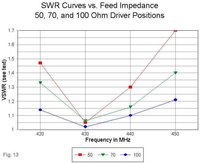
The graph tells an interesting story. At the band extremes, the 50-Ohm impedance driver yields SWR figures sufficient to make one worry about added line losses. This curve results from a large swing in the reactance at the lower impedance--approximately 43 Ohms across the band for a resistance change of only 22 Ohms.
In contrast, the reactance swing of the 70-Ohm driver position is a little over 38 Ohms with a resistance swing of less than 17 Ohms. At the higher impedance, these swings alter the SWR value by a far lower amount than at the 50-Ohm level.
However, for a 50-Ohm main line, I would recommend the 100-Ohm driver position in concert with a 70-Ohm transformation line. The 50-Ohm SWR curve for this arrangement is very flat, with only a 14 Ohm change of resistance and a 6.5 Ohm change of reactance across the band. In general, the higher the feedpoint impedance, the more stable it is across the desired bandwidth. Certainly 300-Ohm feedpoint impedance can be achieved within this general configuration and may be advantageous to some operations.
I have already mentioned the need to complete the development of a satisfactory wire grid arrangement to simulate wire screens in the reflector. Already, someone as asked what the optimal spacing might be for a phased array of corner reflectors, possible for EME work. I shall tackle this problem as soon as 1 GHz CPU computers are available in my price range.
However, there are some interesting lesser phenomena worth investigating as well. The pattern of current peaks along the rods forms a fascinating topography worth some more detailed looks. It will also be interesting to compare this topography to that upon a screen of crossing wires. But all of these questions will have to wait for some available time. In the interim, I hope this much is useful in getting a better grip on the corner reflector.
In the interim, we can at least look at the question of maximum gain that we might obtain by further attempts to optimize this model. In fact, the optimizing efforts expended on this present model were casual, and a more rigorous exploration of dimensions might yield something useful--even if nothing more than a couple of guidelines for manually optimizing models. To that task we turn in Part 3.
Corner refl + dipole: 432 MHz             Frequency = 432  MHz.

Wire Loss: Aluminum -- Resistivity = 4E-08 ohm-m, Rel. Perm. = 1

              --------------- WIRES ---------------

Wire Conn.--- End 1 (x,y,z : in)  Conn.--- End 2 (x,y,z : in)  Dia(in) Segs

1         -5.660,  9.600,  0.000         5.660,  9.600,  0.000 3.75E-01  11
2        -19.000,  0.000,  0.000        19.000,  0.000,  0.000 3.75E-01  31
3        -19.000,  2.000,  2.000        19.000,  2.000,  2.000 3.75E-01  31
4        -19.000,  4.000,  4.000        19.000,  4.000,  4.000 3.75E-01  31
5        -19.000,  6.000,  6.000        19.000,  6.000,  6.000 3.75E-01  31
6        -19.000,  8.000,  8.000        19.000,  8.000,  8.000 3.75E-01  31
7        -19.000, 10.000, 10.000        19.000, 10.000, 10.000 3.75E-01  31
8        -19.000, 12.000, 12.000        19.000, 12.000, 12.000 3.75E-01  31
9        -19.000, 14.000, 14.000        19.000, 14.000, 14.000 3.75E-01  31
10       -19.000, 16.000, 16.000        19.000, 16.000, 16.000 3.75E-01  31
11       -19.000, 18.000, 18.000        19.000, 18.000, 18.000 3.75E-01  31
12       -19.000, 20.000, 20.000        19.000, 20.000, 20.000 3.75E-01  31
13       -19.000, 22.000, 22.000        19.000, 22.000, 22.000 3.75E-01  31
14       -19.000, 24.000, 24.000        19.000, 24.000, 24.000 3.75E-01  31
15       -19.000, 26.000, 26.000        19.000, 26.000, 26.000 3.75E-01  31
16       -19.000, 28.000, 28.000        19.000, 28.000, 28.000 3.75E-01  31
17       -19.000,  2.000, -2.000        19.000,  2.000, -2.000 3.75E-01  31
18       -19.000,  4.000, -4.000        19.000,  4.000, -4.000 3.75E-01  31
19       -19.000,  6.000, -6.000        19.000,  6.000, -6.000 3.75E-01  31
20       -19.000,  8.000, -8.000        19.000,  8.000, -8.000 3.75E-01  31
21       -19.000, 10.000,-10.000        19.000, 10.000,-10.000 3.75E-01  31
22       -19.000, 12.000,-12.000        19.000, 12.000,-12.000 3.75E-01  31
23       -19.000, 14.000,-14.000        19.000, 14.000,-14.000 3.75E-01  31
24       -19.000, 16.000,-16.000        19.000, 16.000,-16.000 3.75E-01  31
25       -19.000, 18.000,-18.000        19.000, 18.000,-18.000 3.75E-01  31
26       -19.000, 20.000,-20.000        19.000, 20.000,-20.000 3.75E-01  31
27       -19.000, 22.000,-22.000        19.000, 22.000,-22.000 3.75E-01  31
28       -19.000, 24.000,-24.000        19.000, 24.000,-24.000 3.75E-01  31
29       -19.000, 26.000,-26.000        19.000, 26.000,-26.000 3.75E-01  31
30       -19.000, 28.000,-28.000        19.000, 28.000,-28.000 3.75E-01  31

              -------------- SOURCES --------------

Source    Wire      Wire #/Pct From End 1    Ampl.(V, A)  Phase(Deg.)  Type
          Seg.     Actual      (Specified)

1           6     1 / 50.00   (  1 / 50.00)      1.000       0.000       V
Updated 4-18-99. © L. B. Cebik, W4RNL. Data may be used for personal purposes, but may not be reproduced for publication in print or any other medium without permission of the author.