

Since my first study in "capacity hats" ("Modeling and Understanding Small Beams: Part 8 Capacity Hats," Communications Quarterly [Fall, 1997], 61-79), a number of questions have come my way. One of the more recent ones is where to place a hat for maximum efficiency (electrically). The answer to the question is quite brief. However, making the answer believable requires an understanding of hats in general. In order to develop an trustworthy answer via modeling on any of the version of NEC or MININEC, let's start by summarizing what may be inaccessible because the original article is not at hand.
2. A hat is an extension of the antenna element. As such, one can read the current curve in continuity with the remainder of that curve on the main element. Depending on the hat structure, the current may divide, but the sum of the individual currents in the hat segments immediately adjacent to the last main element segment is the natural continuity of the main element current curve.
Consequently, the simplest and yet most adequate view of a hat is as a simple mechanical extension of the main element.

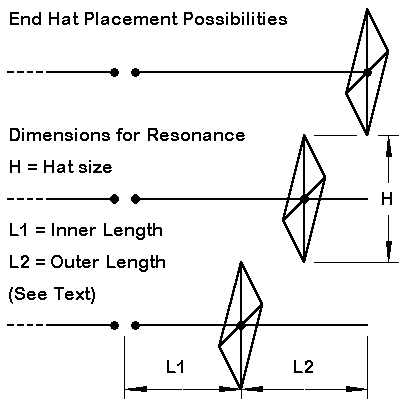
3. Hats come in two general types: symmetrical and non-symmetrical. As shown in the figure, the physical size of each type of hat need not differ to achieve the same goal of bringing a given antenna element to resonance (or to some other specified condition). However, the operation of the two types of hats is quite different.
A non-symmetrical hat provides a single current curve extending from contact with the main element to its end. For variations of shape, see Half-Length 80-Meter Vertical Monopoles: the Best Method of Loading Parts 1-5. The simplest non-symmetrical hat is very likely the inverted L, where the upper horizontal portion of the antenna brings the vertical portion to resonance, but supposedly adds little to the desired pattern. However, as any model will show, the upper portion does radiate and thus has an influence on the overall far field pattern of the antenna.
Symmetrical hats have structures the sum of whose parts yields a cancellation of virtually all radiation. Therefore, they do not contribute more than negligibly to the radiation pattern of the antenna. The main element essentially supplies the far field pattern shape and strength.
4. Of all hat structures and other loading schemes applied to shortened antenna elements, symmetrical hats provide a. the highest gain, b. the highest source impedance, and c. the widest operating bandwidth for both performance characteristics and source impedance. The 80-meter monopole study is a good reference for seeing the relationship of symmetrical hats to various non-symmetrical alternatives with respect to all three categories of antenna properties. However, the following graph can give some indication of the symmetrical hat's superiority to other loading schemes.
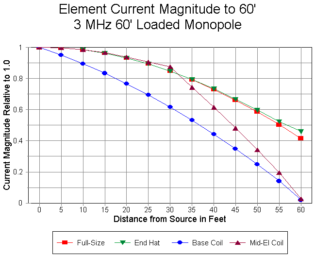
The graph shows the results of modeling 4 antennas. One is a full size monopole over perfect ground, about 78.75' long. The graph carries out the current magnitude curve only to the 60' point, which is the length of the other 3 loaded elements. The full size element, of course, has a current magnitude curve that continues to descend toward a value of zero at the end, and these further portions contribute to the radiation. The shortened elements terminate at the 60' mark.
The current in the symmetrical hat model closely parallels that of the full size antenna up to the 60' point, and in fact slightly exceeds the current of the full-size element at the 60' mark. The mid-element inductively loaded model uses a lossless load. However, the load (253 Ohms) represents a replacement of the main element that would have radiated with a high current magnitude had it been linear. Beyond the load, the element shows a rapid drop in current and a current magnitude curve similar to that appropriate to the low-current-magnitude outer end of a full-size element. The base or source loaded element begins with a rapid drop in current magnitude and descends from that point, even though the load is about half that of the mid-element load (137 Ohms).
The performance of the various models, all with 2" aluminum main elements and referenced to perfect ground, can be seen in this table:
Model               Gain (dBi)          Source Z (R +/- jX)
Full-Size           5.14                36.0 - j 0.1
Hat Load            5.06                31.7 - j 0.1
Mid-XL Load         4.99                25.0 - j 0.5
Base-XL Load        4.97                16.7 + j 0.2
Of course, both forms of loading with inductive reactance would show additional losses once a finite Q is assigned to the inductors. The lesser gain of the reactively loaded elements in these lossless inductor models relative to the hat-loaded element is solely due to the position of the loads and their replacement of high-current magnitude element areas with low-current magnitude areas. Hat losses are already included in the material losses (aluminum) of its structure. It is the superiority of performance promise that brings designers back to the hat as a means of loading shortened elements, despite the obvious mechanical difficulties of implementing this means of loading on either vertical or horizontal elements.
1. Both NEC and MININEC models coincide with each other and with reality. For adequately segmented models, I have seen at most a 2% variance in hat sizes between NEC and MININEC models. Both, in turn, have yielded physical specifications for resonant vertical (monopole) and horizontal (dipole) antenna elements that are well within the normal variances encountered in antenna construction.
Although both NEC-2 and NEC-4 usually show erroneous results when there are angular junctions of wires having dissimilar diameters, this problem tends to disappear when the radiation field from one of the elements or element sets is self-cancelling. Symmetrical hats meet this requirement. Moreover, even non-symmetrical hats, where there is considerable radiation cancellation due to the physical layout, provide usable guidance in the construction of a physical version of the model.
Consequently, NEC and MININEC models are generally trustworthy, especially for analyzing trends in hat construction variables that are treated systematically.
2. For many studies of trends, modeling monopoles over perfect ground is a compact method of investigation. Since the NEC and MININEC modeling systems create an image antenna, they replicate what one might construct for a hatted dipole in free space, but with half the required segments. This move, in turn, permits high segmentation density for maximum accuracy and for reading out small changes in current along the length of the elements, all without exceeding a programs total segment count limit or without incurring long run times.
A monopole over perfect ground will bear the following relationships to an equivalent dipole in free space. a. The free space dipole will be exactly twice as long as the perfect-ground monopole. NEC models should use an odd number of segments in the dipole to permit exact center-placement of the source.

b. The source impedance of the monopole will be half the source impedance of the dipole. The figure might be slightly off in a NEC pair of models because the source position of the monopole is in the middle of the first segment above ground, while the dipole source is perfectly centered. With adequate segmentation, the differential will be insignificant.
c. As shown in the figure, the monopole gain will be 3 dB higher than that of the free space dipole due to the reflection of the ground. Hence, for calculating the gain of a horizontal dipole over a ground with a known reflection gain, one simply subtracts 3 dB from the monopole gain and then adds the appropriate reflection gain for a final value.
In all of this, the use of monopoles over perfect ground is perfectly adequate to tracking trends of performance and of changes to the hatted antenna's structure. Essentially, the difference between the perfect- ground monopole and antennas at heights over real ground are a set of arithmetic constants.
For another study, I ran models of a 16-meter long vertical monopole at 3 MHz with a variety of wire hats ranging from 3 to 32 spokes and using 2 different designs. One design used only spokes, while the other used spokes plus a perimeter wire that connected the spoke tips. In every case, the length of the spokes and other hat dimensions were adjusted for resonance over perfect ground. The figure shows a few of the possible variations, but not to scale.

We can show the performance of the various hats in a pair of tables. First, the models using only spokes:
Number         Spoke-Length        Gain           Source Z
of Spokes      Meters              dBi            R +/- jX Ohms
 3             5.994               4.96           27.9 _ j 0.7
 4             4.966               4.98           27.8 - j 0.7
 6             3.848               4.99           27.9 + j 0.4
 8             3.239               4.99           27.9 + j 0.4
12             2.611               5.00           27.9 - j 0.2
16             2.297               5.00           27.9 - j 0.9
24             2.007               5.00           27.9 - j 0.3
32             1.861               5.00           28.0 - j 0.2
For models using a spoke-plus-perimeter-wire construction, the table looked like this:
Number         Spoke-Length        Gain           Source Z
of Spokes      Meters              dBi            R +/- jX Ohms
 3             2.985               4.97           28.1 + j 0.1
 4             2.591               4.98           28.1 + j 0.6
 6             2.280               4.99           28.0 + j 0.8
 8             2.096               4.99           27.9 - j 0.5
12             1.918               5.00           28.0 + j 0.1
16             1.808               5.00           27.9 - j 0.8
24             1.701               5.00           27.9 - j 0.3
32             1.640               5.00           28.0 - j 0.2
Clearly, there is no significant difference in the source impedance regardless of the hat construction method or the number of spokes in the hat structure. Likewise, there is a maximum difference of 0.04 dB in the gain figures. The only difference of significance is the length of the spokes, which define a virtual "radius" for the various hat structures.
One cannot combine all of the hats into a single graph, since there are two different geometric progressions at work. However, we can graph one of the progressions. Let us use the 4-8-16-32 spoke progression.

As the graph shows, there is a regular curve to the reduction of spoke lengths as the number of spokes increases. The spoke-plus-perimeter-wire hat form effects large size reductions for low spoke number structures. You can estimate the reduction by considering that the true element end is not a spoke tip, but instead a point along the perimeter wire halfway between spoke tips. Adding this length to the spoke length very roughly approximates the spoke length of the counterpart spoke-only design. As the number of spokes increases, the distances between spoke tips shrinks, bringing the two designs closer to coincidence of effective radius.
At some point beyond the right edge of the graph, the curves for the spoke- only and the spoke-plus-perimeter-wire design will come together. At that same point, the addition of further spokes will not significantly decrease the radius of the hat further. In effect, the hat will simulate a solid surface.
What distinguishes wire and disc hats from other symmetrical hat forms, such as the cylinder, is the fact that wire and disc hats have no linear dimension along the axis of the main linear element. Cylinders have such a linear dimension, and as such actually comprise less a hat structure than a change of element diameter, even if the change is very large.
In the exercise just noted, the main element and the hat wires had different but constant diameters. However, there are some hat size variations occasioned by changes in the ratio of the main element diameter to the hat wire diameter. To sample these variations, let us use a 60' long monopole over perfect ground, but change its diameter in regular steps from 0.5" to 2.0". Then, let us use different size wires for the hat structure. #12 AWG (0.0808"), 0.25", and 1" hat wire diameters will suffice for illustration.
We shall explore two hat structures. One is a 4-spoke (only) hat, and the other is a 4-spoke-plus-perimeter-wire hat. Let's record the required spoke lengths for each type of hat throughout the combinations of main element diameters and hat wire diameters.
#12 AWG (0.0808") diameter hat wire
Element Diameter         Spoke-Only          Spoke + Perimeter
in inches                Length - inches     Length - inches
     0.5                  99.2               57.2
     0.75                103.8               60.0
     1.0                 107.4               62.1
     1.25                110.4               63.9
     1.5                 112.9               65.4
     1.75                115.1               66.7
     2.0                 117.1               67.9

0.25" diameter hat wire
Element Diameter         Spoke-Only          Spoke + Perimeter
in inches                Length - inches     Length - inches
     0.5                  90.3               54.0
     0.75                 94.9               56.8
     1.0                  98.4               58.9
     1.25                101.3               60.7
     1.5                 103.7               62.2
     1.75                105.9               63.5
     2.0                 107.9               64.7

1.0" diameter hat wire
Element Diameter         Spoke-Only          Spoke + Perimeter
in inches                Length - inches     Length - inches
     0.5                  77.4               49.6
     0.75                 81.8               52.3
     1.0                  85.2               54.4
     1.25                 88.0               56.1
     1.5                  90.3               57.6
     1.75                 92.4               58.9
     2.0                  94.3               60.1

The first graph shows the same data as in the table, but makes clear the regularity involved. For the spoke-only design, where the hat wire is a constant diameter, the greater the ratio of main element diameter to hat wire diameter, the larger the required spoke length or hat radius.

The second graph shows essentially the same story for the spoke-plus- perimeter hat design. Even for this design, with naturally shorter spokes, the increases are significant.
Interestingly, there is no significant difference in the main element current magnitude in the segment adjacent to the junction with the hat structure, regardless of element diameter. For a #12 wire hat diameter, the current magnitude (relative to 1) in the last main element segment for a 0.5" diameter element is 0.463 and for a 2.0" diameter element is 0.464, both for 60' long elements. The first segments in the 4 spokes show 0.110 and 0.111, respectively for the two element diameters. The longer spokes, however, do show a slower decrease in current, as one might expect, since the terminating value is zero in both cases.
The original question was whether it makes a difference where along a shortened element one places a hat, so long as the hat is generally out toward the end somewhere. The answer is yes. For any given combination of main element length and diameter and a given hat wire diameter, where the hat is sized to achieve resonance (or some other specified condition), end placement is always electrically the most efficient. Any other placement requires either a. for a constant hat size, a lengthening of the overall element, or b. for a given element length, an increase in the hat size. Moreover, every alternative position yields less gain than an end hat, although option b. with the set length and growing hat yields less gain than a constant hat size and lengthening element.
To reach this conclusion, I ran a series of models, of which we shall sample just a few. Consider a 60' long 3 MHz vertical element over perfect ground with an end hat. Then in successive steps (we shall use 5' steps), move the hat down. Then check resonance and a. increase the element length to achieve it or b. increase the hat size to achieve it.
Hat Place      Element        Spoke          Gain      Feed Z
               Length "       Length "       dBi       R +/- jX
End Hat        720            109            5.06      31.7 - j 0.1
5' Down        720            127            5.03      29.4 - j 0.9
               782            109            5.04      30.3 + j 0.6
10' Down       720            144            5.00      27.2 + j 0.1
               808            109            5.04      29.3 + j 0.6
15' Down       720            160            4.97      24.8 - j 0.9
               830            109            5.04      25.5 + j 0.5
Clearly the movement of the hat inboard relative to the element end demands an increase in one or another dimension to restore resonance. Lengthening the element itself beyond the hat maintains the higher gain, but at the expense of ending up with little or no saving in element length, which was the initial motivation for hat loading in the first place. (A full-size element is about 945" long.) The constant length element has a decreasing gain curve, but a rapidly enlarging hat radius--nearly 50% in the example.
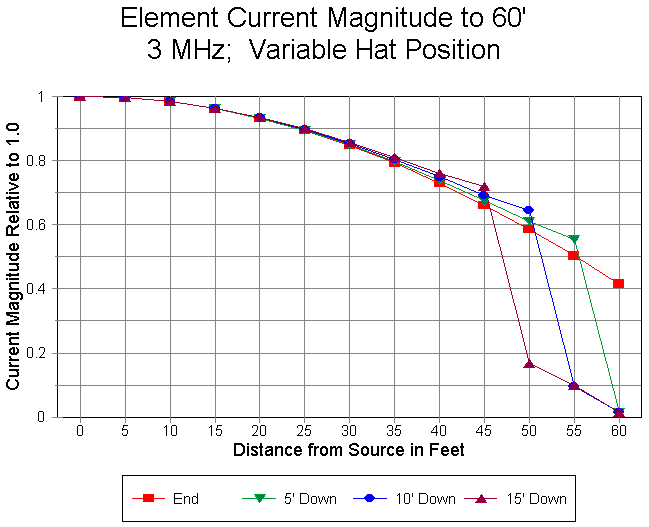
The relative futility of moving the hat inboard relative to leaving it at the element's end appears in current graphs of the constant-length models in this sequence. The hat occupies a significant length of main linear element, wherever it appears. The current levels beyond the hat are those appropriate to a linear element's end, and thus have little current to contribute to radiation. Placing the hat at the outermost point along the element allows it to function with the smallest size and to occupy the element portion with the lowest current (relative to any other possible position).
The exact dimensions, hat growth, and wire length growth will, as noted vary with the exact set of structural dimensions chosen. However, the trend will not change. Whatever the mechanical difficulties involved, hats are physically smallest and electrically most efficient (or detract least from the antenna's performance) when located at the outermost limit of a proposed antenna element. This applies not only to vertical monopoles, but as well to dipole structures. Perhaps the only two operative reasons for placing a hat inboard on a monoband antenna are these: a. the inboard placement is mechanically dictated by support requirements; b. the inboard hat placement is designed solely to change the frequency of a secondary resonance of the element.
The conclusions prompted the the modeling survey have been for a long time a part of antenna lore, which is replete with tales of silly things people supposedly have done, like clipping off the wire remnant from someone's hatted mobile whip. The claim was that the unrequested modification did not adversely affect radiation. However, as the table shows, it did adversely affect radiation--although in a minuscule manner--and, more significantly, it did affect system resonance. The clipping culprits in this legend turned out to be only 1 fact less ignorant than the victim of their (undoubtedly Halloween) vandalism.
Legends aside, these exercises in modeling do more than set up an additional support for placing hats as far outboard as the antenna's physical structure permit. They provide a body of data about source impedance, gain, and current magnitude along the element to clarify somewhat the overall understanding of hat properties. The project has been as much an exercise in using all of the data provided by modeling programs as it has been a demonstration of hat properties. (There is, in fact, further data available that goes beyond the scope of this particular set of notes.)
Time to go. Now where did I leave mine--hat, that is. It was hanging on the end of an antenna when I came in.
Updated 10-31-98. © L. B. Cebik, W4RNL. Data may be used for personal purposes, but may not be reproduced for publication in print or any other medium without permission of the author.