
 A 10-Meter LPDA
1. A full-size 2-element Yagi, with just over 6 dBi free space gain requires a boom at least 5' long if it is to cover most of the 28 to 29.7 MHz span. However, front-to-back ratio will be quite low, average between 10 and 11 dB.
2. Small 2-element beams with better front-to-back ratios, such as the Moxon rectangle (15-30 dB across much of the band), have slight lower gain figures and rarely cover the entire band with consistent gain and front-to- back ratios.
3. ZL-Special/HB9CV antennas can raise the free space gain to about 6.5 dBi peak, with a peak front-to-back ratio of about 20 dB. However, they cover a little more than 1 MHz of the band.
4. 3-element Yagis, while providing more gain, are limited in a number of ways. For high gain (8 dBi), one needs a 12' boom. With an 8' boom, the gain peaks at just over 7 dBi, and the bandwidth is less than 1 MHz. Orr and Reisert designs can cover the band at the 7 dBi peak gain figure, but require something close to a 12' boom.
5. 2-element quads are capable of about 7 dBi peak gain and about 20 dB front-to-back ratio, but lose most of their gain and front-to-back ratio when pressed beyond about 1 MHz of 10-meter coverage.
One can dream up other contenders in the contest for adequate gain, good front-to-back ratio, and full-band coverage, but almost all tend to show severe roll-offs in gain and front-to-back when pressed beyond about 1 MHz of 10 meters. All but one, that is.
It is possible to design--at least in principle--a 10-meter array on an 8' boom that will provide very consistent 7 dBi free space gain and 20+ dB coverage across 10-meters with a flat SWR well below 1.5:1. The design is a monoband log-periodic dipole array (LPDA). The ARRL Antenna Book has carried a K1TD monoband 2-meter design for a number of years (pages 10-17 to 10-19 in the 18th Edition). Jerry Hall's design had to cover a 2.75% frequency range, while a 10 meter LPDA would have to cover a 6.9% frequency range. But the project seemed feasible on paper.
Requirements for the antenna are a free space gain at or close to 7 dBi across the band with a 20 dB or better front-to-back ratio. The design would have to fit on an 8' boom to meet my preconception of compactness. Here are some practical notes on what I have encountered so far in this unfinished business. (The theory and design notes in The ARRL Antenna Book and other basic references, such as Johnson and Jasik, are essential background reading in Log Periodic Dipole Arrays (LPDAs). I shall not go into that material here.)
The designs were cross checked on NEC-4, using linear elements and the TL function to simulate the element-to-element reversing antenna transmission line. I believe that LPDA models using this technique are reasonably accurate when they have elements with a uniform diameter. LPCAD provides a source impedance estimate that holds up quite well in NEC-4 models. All models were designed for a 200-Ohm antenna transmission line. Although the software recommends a 4:1 balun at the feedpoint, the recommendation is not wholly consistent with the projected (and modeled) source impedances for various versions of the antenna. For various models, I achieved a relatively flat SWR curve for a 50-Ohm system feedline cable by employing matching sections of 75-Ohm and 93-Ohm cable for source impedances in the 100 to 145-Ohm range. The basic design of these sections is the quarter wavelength, but the actual lengths were adjusted to compensated for remnant reactance. This matching system, of course, would not be apt to a wide-band LPDA, such as a 20-10-meter antenna. However, it suits the needs of the monoband design.
Initial models based on software generated designs showed that if I specified a frequency range of 28 to 30 MHz, most of the higher gain and front-to-back figures occurred at the uppermost portion of the range and beyond. For 0.5" linear elements, satisfactory NEC-4 modeling results were achieved by specifying a range of 27.5 to 29.5 MHz, about 2% low at both ends. The software uses an upper-end frequency buffer to ensure high frequency performance. At the lowest frequency selected, the element length is calculated according one of three element length-to-diameter ratios, the highest value limit being equal to or greater than 105. The longest element in this example has a ratio of over 400:1. (My thanks to Roger Cox, the software author, for providing the lower frequency calculation numbers.) Hence, it is reasonable that the rear element length would show up as short in the initial calculations.
Once a satisfactory model had emerged using uniform-diameter 0.5" elements, the model was converted to 108" center sections of 0.5" diameter aluminum with 0.375" diameter outer sections--in prospect of building an actual antenna one day. The conversion resulted in a degradation of modeled performance until the ends of the rearmost element were shortened by about 3.5" each. The following, with an exception to be noted, is the EZNEC-4 model description of the semi-frozen design.
lpda10m:  tapered element design   Frequency = 28 (to 30) MHz.
Wire Loss: Aluminum -- Resistivity = 4E-08 ohm-m, Rel. Perm. = 1
              --------------- WIRES ---------------
Wire Conn.---End 1 (x,y,z : in)  Conn.---End 2 (x,y,z : in)   Dia(in) Segs
1         0.000,-106.00,  0.000  W2E1   0.000,-54.000,  0.000 3.75E-01  10
2  W1E2   0.000,-54.000,  0.000  W3E1   0.000, 54.000,  0.000 5.00E-01  23
3  W2E2   0.000, 54.000,  0.000         0.000,106.000,  0.000 3.75E-01  10
4        35.605,-98.003,  0.000  W5E1  35.605,-54.000,  0.000 3.75E-01   8
5  W4E2  35.605,-54.000,  0.000  W6E1  35.605, 54.000,  0.000 5.00E-01  23
6  W5E2  35.605, 54.000,  0.000        35.605, 98.003,  0.000 3.75E-01   8
7        67.475,-87.720,  0.000  W8E1  67.475,-54.000,  0.000 3.75E-01   6
8  W7E2  67.475,-54.000,  0.000  W9E1  67.475, 54.000,  0.000 5.00E-01  23
9  W8E2  67.475, 54.000,  0.000        67.475, 87.720,  0.000 3.75E-01   6
10       96.000,-78.515,  0.000 W11E1  96.000,-54.000,  0.000 3.75E-01   4
11W10E2  96.000,-54.000,  0.000 W12E1  96.000, 54.000,  0.000 5.00E-01  23
12W11E2  96.000, 54.000,  0.000        96.000, 78.515,  0.000 3.75E-01   4
13      150.000, -0.200,  0.000       150.000,  0.200,  0.000    # 14    1
             -------------- SOURCES --------------
Source    Wire      Wire #/Pct From End 1    Ampl.(V, A)  Phase(Deg.)  Type
          Seg.     Actual      (Specified)
1           1    13 / 50.00   ( 13 / 50.00)      1.000       0.000       I
No loads specified
                -------- TRANSMISSION LINES ---------
Line  Wire #/% From End 1   Wire #/% From End 1  Length      Z0    Vel Rev/
      Actual  (Specified)   Actual  (Specified)             Ohms  Fact Norm

1    2/50.0  (  2/50.0)    5/50.0  (  5/50.0)  Actual dist  200.0  1.00  R
2    5/50.0  (  5/50.0)    8/50.0  (  8/50.0)  Actual dist  200.0  1.00  R
3    8/50.0  (  8/50.0)   11/50.0  ( 11/50.0)  Actual dist  200.0  1.00  R
4   11/50.0  ( 11/50.0)   13/50.0  ( 13/50.0)   80.000 in    75.0  1.00  N
5    2/50.0  (  2/50.0)  Short ckt (Short ck)   36.000 in   200.0  1.00
Ground type is Free Space
Wires 1-12 are the 4 elements, while wire 13 is a short segment used as a source point for the far end of the 80" (VF=1) section of 75-Ohm cable (TL #4). TL #5 is not part of the original design, but is part of a modified model to be discussed later. I include it here, since there are few change made to the original model, and reproducing the entire wire table further down seems unnecessary.
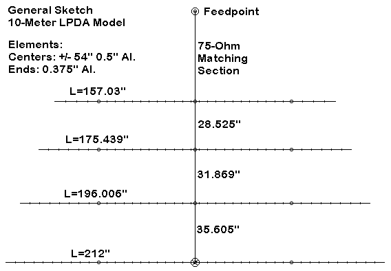
The figure shows graphically what the table reveals in detail. LPCAD had specified end lengths of +/- 109.448" (nearly 219" overall) for the rear element, which was reduced to +/- 106" (212") in the model for enhanced modeled performance.

The free space azimuth patterns give a reasonably clear picture of anticipated performance from the antenna. Gain is remarkable consistent across the band, and the front-to-back ratio meets the goal of 20 dB or better across the band. Hence, the basic goal of the exercise (apart from the question of whether the antenna can be reasonably home-brewed) has been met.
So I tried several lengths of stubs, ranging from 1" (simulating a practical short across the rear of the antenna transmission line) to 52". Here is a quick table of modeled performance figures for 28.5 MHz with various stub lengths:
Stub Length    Gain dBi  F-B dBi   Source Z       Notes
(inches)                           (R+/-jX)
  1            7.18      21.14     43.1 - j 9.7
  6            7.16      27.11     43.6 - j 6.4
 12            7.13      34.78     43.9 - j 4.3   Max F-B at 28.0 MHz
 18            7.11      45.47     44.2 - j 3.2
 24            7.09      40.92     44.4 - j 2.4
 30            7.08      36.13     44.5 - j 1.8
 36            7.07      33.57     44.6 - j 1.4   Max F-B at 28.7 MHz
 42            7.07      31.94     44.7 - j 1.1
The chief effect of using stubs of different lengths is to move the frequencies of maximum gain and of maximum front-to-back ratio, with shorter lengths moving those frequencies lower. There is a general increase in both the gain and the front-to-back ratio at the test frequency, although it may be somewhat marginal in actual operation.
With exceedingly short stubs (1 to 12"), the gain at 28 MHz increases--up to 7.5 dBi for the shortest stub that simulates a near direct short circuit. However, three factors suffer. First, the gain across the band becomes quite unequal, with the gain at 30 MHz no higher than for any of the stub lengths. Second, the front-to-back ratio at 28 MHz drops below 20 dB. Third, the source impedance at 28 MHz falls outside the matching range of the matching section, with an increase in SWR to about 2:1 with a 1" stub.
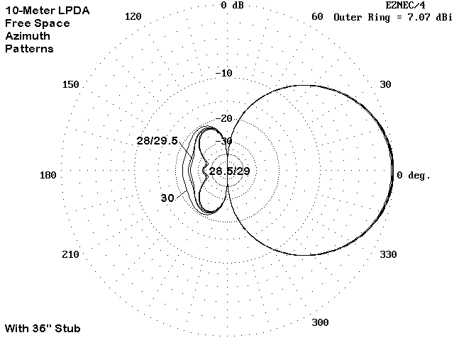
The figure shows the free space azimuth patterns of the array across the 28-30 MHz span with a 36" stub added to the original model. The improved front-to-back ratios are apparent.
The following figures graph performance for the model using a 212" rear element and having either no stub (open) or a 36" stub. These figures use the red and green lines; ignore the blue line in each chart for the moment.
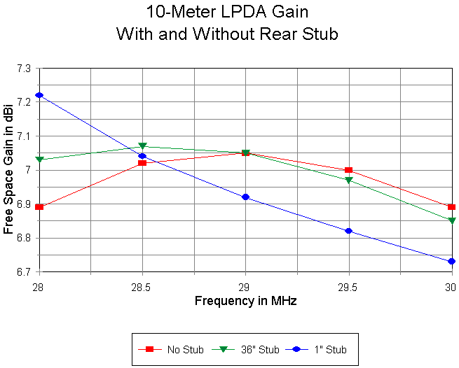
The gain values and peak positions appear best in graphs like the one above. Clearly apparent is the displacement of the gain curve lower in frequency relative to the open-ended model. Since this model uses tapered- diameter elements, the gain figure is likely about 0.05 dB high everywhere on the graph. This over-report of gain is an estimate based on the modeled performance with uniform 0.5" diameter elements. It is not possible to model this antenna with the tapered-diameter correction factor active for every element, since the shortest element falls outside the +/-15% natural resonance limitation. Hence, models with the feature activated will only correct a maximum of 3 of the 4 elements.
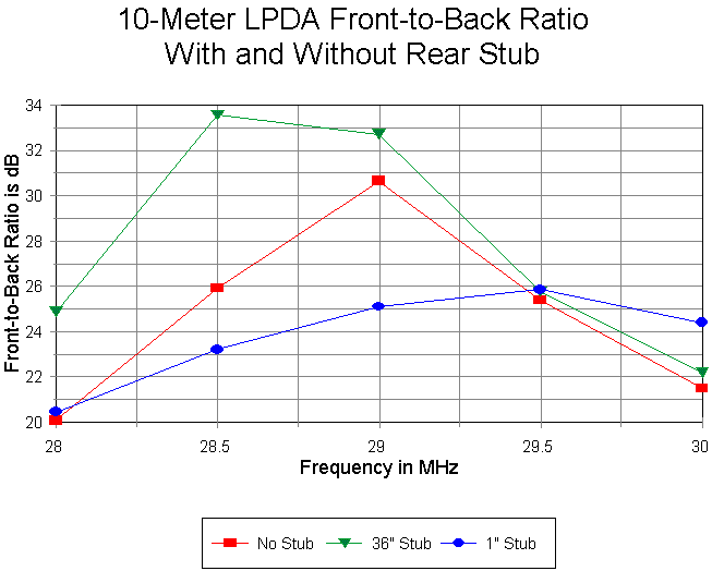
The increase in overall front-to-back ratio, plus the displacement of the curve lower in frequency, also appears most clearly in a graph like the one above. Relative to a MININEC model, it is likely that both curves may suffer about a 50 kHz displacement higher in frequency due to the tapered- element diameters.
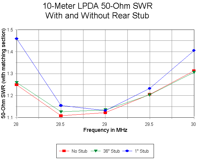
Adding the 36" stub has virtually no effect on the post-matching section 50-Ohm SWR curve. Either version of the modeled antenna provides among the flattest curves obtainable over a 2 MHz span. However, as noted, the use of a very short stub will displace the SWR curve at the lower end of the band covered.
The advisability of the termination for the antenna transmission line is a mixed bag. The improvements in performance are desirable. However, an additional 3' of transmission line extending from the rear of the antenna might physically defeat the antenna's claim to compactness.
Let us remember, however, that the open-end model had its rear element optimized for this application. It might be possible to change the rear element length to a value optimized for the use of the 1" (simulated short) at the rear. I finally settled on a value of 215" (+/- 107.5") for the rear element--longer than the open-rear model and shorter than the LPCAD recommended length.
The blue lines on the three graphs above show the results of using this longer element with a 1" stub. The length of the matching line (TL #4) was increased to 90" to center the SWR curve across the band.
Adding a direct short or a very short stub to the rear of the antenna transmission line changes the gain curve of the antenna. Although the peak value at 28 MHz exceeds either of the other models, the gain rapidly decreases (relative to LPDA design, but not necessarily to other phased arrays or to Yagis) so that the 30-MHz end value is noticably lower than the other LPDA models. The front-to-back curve, on the other hand, is almost without peak compared to other LPDA models, with a smoother curve across the band and always above the 20 dB design goal value. The SWR curve, while steeper than those of the other LPDA models, is still very good, with no point reaching 1.5:1.
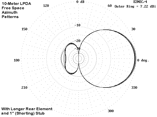
The revised ("blue-line") model, whose free space azimuth patterns appear in the figure above, overcomes the need for a long stub. However, the gain and SWR curves are not so well behaved as those of the open-end model. Hence, the ultimate decision of which design to use still rests on a judgment of which characteristics are most important to the builder. At this point in the design work, I suspect--but do not know for certain--that judicious element length or spacing changes might smooth out the gain curve without jeopardizing other factors, but obviously, the first order design techniques lose their ability to guide these efforts.
Using #12 AWG copper wire as the material of choice, the length-to-diameter ratio of the elements exceeds 2000:1. Nonetheless, let's look at a preliminary model of a wire LPDA for the 10-meter band.
lpda10m:  #12 AWG wire   Frequency = 28 (to 30)  MHz.
Wire Loss: Copper -- Resistivity = 1.74E-08 ohm-m, Rel. Perm. = 1
              --------------- WIRES ---------------
Wire Conn.---End 1 (x,y,z : in)  Conn.---End 2 (x,y,z : in)   Dia(in) Segs
1         0.000,-111.52,  0.000         0.000,111.520,  0.000    # 12   43
2        35.619,-99.776,  0.000        35.619, 99.776,  0.000    # 12   41
3        67.488,-89.269,  0.000        67.488, 89.269,  0.000    # 12   39
4        96.000,-79.869,  0.000        96.000, 79.869,  0.000    # 12   37
5       150.000, -0.200,  0.000       150.000,  0.200,  0.000    # 14    1
              -------------- SOURCES --------------
Source    Wire      Wire #/Pct From End 1    Ampl.(V, A)  Phase(Deg.)  Type
          Seg.     Actual      (Specified)
1           1     5 / 50.00   (  5 / 50.00)      1.000       0.000       I
No loads specified
                -------- TRANSMISSION LINES ---------
Line  Wire #/% From End 1   Wire #/% From End 1   Length     Z0    Vel Rev/
      Actual  (Specified)   Actual  (Specified)              Ohms Fact Norm
1    1/50.0  (  1/50.0)    2/50.0  (  2/50.0)  Actual dist  200.0  1.00  R
2    2/50.0  (  2/50.0)    3/50.0  (  3/50.0)  Actual dist  200.0  1.00  R
3    3/50.0  (  3/50.0)    4/50.0  (  4/50.0)  Actual dist  200.0  1.00  R
4    4/50.0  (  4/50.0)    5/50.0  (  5/50.0)   80.000 in    93.0  1.00  N
Ground type is Free Space
In order to center the operating characteristics of this antenna within the 28-30 MHz spran, it was necessary to lower the lower and upper design limit frequencies fed to LPCAD to 27 and 29 MHz, respectively. Hence, all elements are longer than for the tubing model version.
The source impedance for this version of the LPDA increased from the 120- Ohm region to the 140-Ohm region. Hence, the 75-Ohm matching section was replaced with a 93-Ohm section, simulating RG-62, but without the velocity factor being taken into account (an easy calculation during construction). The matching section used here provides SWR curves very much like those for the model using aluminum tubing.
For a general picture of the anticipated antenna performance, we may look at the free space azimuth patterns below.
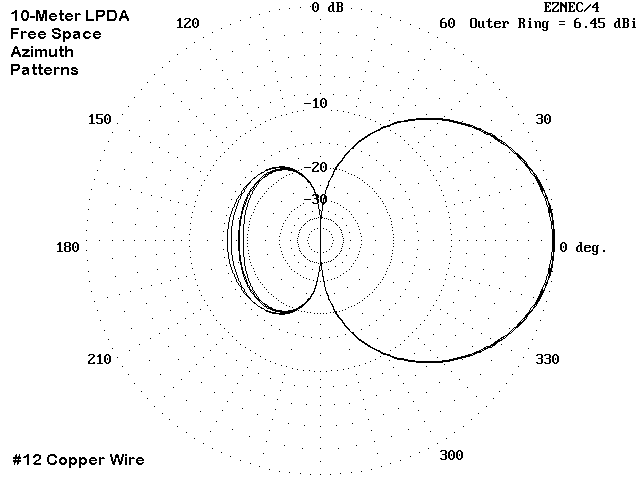
Clearly apparent are the overall reduce gain of the wire antenna in this configuration, as well as the well-controlled but lower values of front-to- back ratio.
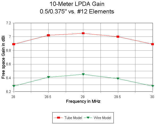
How the gain curve compares to the tapered-diameter tubing version of the antenna is clearest on a graph that separates each frequency.
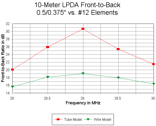
Comparable front-to-back curves appear in the graph above.
The overall gain and front-to-back curves, although covering the entire 10- meter band, are closer to what an HB9CV antenna might achieve with fewer elements and a shorter boom (but with a narrower operating bandwidth for both the SWR and the antenna characteristics). They are shy of short-boom 3-element Yagi performance by a good bit.
These results do not condemn wire LPDAs. However, they do show that the methods of calculating elements optimized for much lower length-to-diameter element ratios do not yield the same results when translated to wire elements. In short, further research into the calculation methods--or plain old modeling cut and try--will be needed to arrive at a higher performance model--if one is possible for the given boom length.
Programs like LPCAD are valuable tools in the design process. They automate most of the initial calculation work, as well as a good portion of the re-calculation work. However, one must supplement them with as good a set of models as the current cores will permit. NEC-2 is entirely adequate for uniform-taper elements, but even NEC-4 must be used with caution when moving to tapered-diameter elements.
The original goals of the project were met early on. The open-rear tubing version of the antenna yields a consistent gain close enough to that of a short-boom 3-element Yagi to serve the purpose, and the front-to-back ratio exceeds 20 dB across all of 10 meters. The operating bandwidth--including both the SWR and the antenna characteristics--is clearly superior to anything else I have seen on the same length of boom.
However, every project raises as many questions as it answers. So besides leaving some unsettled matters concerning construction methods that might be replicated in the average home workshop, there are a number of questions regarding LPDA calculations for thin elements to be researched, a number of rear stub versions to be optimized, and a number of other questions that likely will not be known until they crop up in the supplemental work.
When I learn more, I'll add to these notes. I hope what is here is useful.
Updated 11-08-98. © L. B. Cebik, W4RNL. Data may be used for
personal purposes, but may not be reproduced for publication in print or
any other medium without permission of the author.