A trap consists of an inductance and a capacitance, normally resonated just at or below the lowest frequency of the higher antenna frequency range. The limiting factor in a trap is the resistive loss of the coil, since the losses in capacitors at HF are very small. A trap effectively consists of a series combination of resistance and inductive reactance in parallel with capacitive reactance. See Figure 2a.

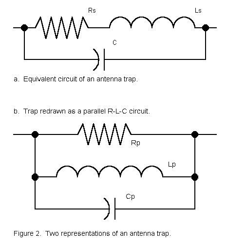
Unfortunately, we cannot directly model the situation in Figure 2 as a lumped constant load. NEC loads permit series R-L-C combinations, parallel R-L-C combinations, or series R-X combinations. It is necessary therefore, to convert the complex series-parallel circuit into an equivalent parallel R-L-C circuit, as illustrated in Figure 2b. However, since this procedure requires the transformation of component values into reactances, the conversion is frequency specific. Therefore, modeling a trap requires separate calculations and models for each frequency band of interest.

To do an actual calculation, we require some one of the following combinations of data:

a. The inductance and Q of the coil, the capacitance, and the frequency of interest;

b. The inductive and capacitive reactances, the resistance, and the frequency of interest; or

c. The inductive and capacitive reactances, the coil Q, and the frequency of interest.

Using measurements made by Roger Cox, WB0DGF, of commercial traps, we can consider a 15-meter trap that consists of a 3.3 µH coil with a Q in the range of 235. For resonance at 21 MHz, the coil requires a capacitance of about 17.4 pF.

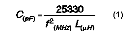
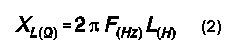
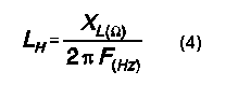
With the given Q, the series resistance of the coil requires that we find the reactance of the coil at 21 MHz. By the standard formula, the reactance is about 436 ohms.

Dividing the reactance by Q, we get a resistance of about 1.9 ohms.

To convert the series R-L into a parallel R-L combination, we use the standard conversion equations:

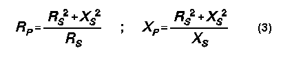
The equations give these values: XL = 436 ohms; R = 100,000 ohms. The corresponding value of L comes from the reverse of equation (2):

The parallel inductance value will be 3.3 µH. We now have our parallel R- L-C trap load for operation at 15 meters.

At 20 meters, we may also calculate the requisite values of parallel R and L. The 3.3 µH inductance has a reactance of about 292 ohms. Dividing this reactance by the Q, which we assume to remain fairly constant, the series resistance is 1.25 ohms. The parallel equivalents are these: XL = 292 ohms; R = 67,300 ohms. The inductance of this parallel combination is 3.3 µH. The capacitance remains at 17.4 pF.

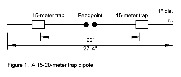
To model the trap dipole at 21.2 MHz and 14.1 MHz (as sample frequencies), we can create a model using a 1" diameter aluminum element with the following wire limits of the X coordinate (where both the Y and Z coordinates remain "0" for a free space model):

          Wire      End 1          End 2          Segments
          1         -13.67         -11.3             8
          2         -11.3          -10.8             1
          3         -10.8           10.8            41
          4          10.8           11.3             1
          5          11.3           13.67            8

We place a parallel R-L-C load in elements 2 and 4. These short wires, no longfer than a single segment of adjacent wire, permit independent adjustment of the antenna length for the two bands in question. For 21.1 MHz, the R-L-C values are expressed in the form most used by implementations of NEC: 1E05, 3.3E-06, 17.4E-12. For 14.1 MHz, the R-L-C values are 6.73E4, 3.3E- 06, 17.4E-12. The length of the trap is absorbed by the overall antenna element lengths. Slight differences in diameter for the short trap lengths at the current levels in the region of the traps are not significant variables, relative to real installations: ground clutter will create larger variations than trap diameters. A possible exception are dual-trap assemblies, which may be directly modeled as a larger wire diameter between traps. Use of shorted stubs as inductors also make no difference since, in principle, these radiate even less than solenoid inductors.

For comparison purposes, model dipoles were constructed of the same 1" diameter aluminum tubing, but without traps. The 14 MHz dipole was 33.3' long at resonance, while the 21.2 MHz dipole was resonant when 22' long. Both dipoles showed a free space gain of 2.13 dBi with a feedpoint impedance of 72 ohms.

The 21.2 MHz trap-loaded dipole showed a free space gain of 2.06 dBi, a mere 0.07 dB less than the trapless dipole. The feedpoint impedance was 73.9 ohms. The trap showed an impedance of 5175 - j22155 ohms, effectively terminating the antenna. Current levels beyond the traps were not significant, never rising above 2.5% of the source current.

In contrast, the 14.1 MHz trap-loaded dipole (trap resonant at 21.0 MHz) showed a free space gain of 1.87 dBi, 0.26 dB less than its trapless counterpart, with a feedpoint impedance of 66.2 ohms. The reduction in gain is partly due to the shortening of the overall dipole length.

However, the parallel R-L-C equivalent of the trap also plays a role in the gain reduction. We may derive a value for the trap's Q by reversing our calculations and deriving a set of series values for R and XL. The net parallel reactance of the trap at 14.1 MHz is given by the equation:

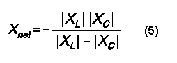
Using the resultant value of parallel reactance, 532 ohms, and the 63.7 kohms parallel resistance, we may calculate equivalent series values of resistance and reactance from standard equations:

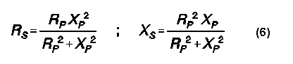
The calculated series values are these: R = 4.2 ohms; XL = 532 ohms. (These values are autiomatically calculated by NEC and appear as part of its output data.) Dividing XL by R, we derive a Q of approximately 126 at 14.1 MHz. Note that this value varies from the expectation of those who wish to discount the capacitor and reduce the trap to a simple series combination of resistance and inductive reactance. NEC data suggests that the losses in the trap at 14.1 MHz are approximately double the losses at 21.2 MHz.

An equally shortened 14.1 MHz dipole with a center loading coil requires an inductive reactance of 174 ohms to be resonant. A lossless center coil yields a dipole free space gain of 2.00 dBi. Only by adding a series resistance of 1.2 ohms can the free space gain of the dipole with 15-meter traps (1.87 dBi) be replicated. The Q of the equivalent center loading coil thus becomes about 145.

The lower the frequency below the resonant frequency of the trap, the higher the Q of a given trap. At some very low frequency, lower than 1/10th the resonant trap frequency, the trap Q very closely approaches the initial Q of the coil (assuming that the initial Q is valid at that distant a frequency, which is dubious). Q of the trap assembly is lowest at resonant frequency. Hence, a 10-meter trap may show a higher Q at 20 meters than at 15 meters.

Experience has shown that the losses in gain of center loaded elements are additive, at least in 2-element Yagis. If this experience holds true of the 14.1 MHz elements with 15-meter traps, then one might expect about 0.5 dB loss of forward gain relative to a full size Yagi of the same design but unloaded.

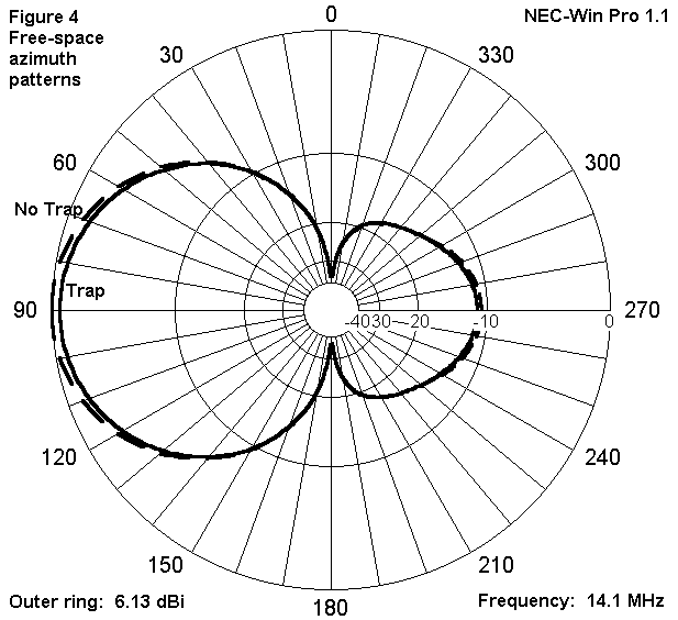
To test this hypothesis, I scaled a 10-meter beam with a 50-ohm feedpoint impedance for 14.1 MHz. The new full-size beam spaced the elements by 12.12', again using 1" aluminum tubing for modeling simplicity, as shown in Figure 3. With a driven element 32.2' long and a reflector 34.94' long, the beam achieved its maximum front-to-back ratio (10.68 dB), a figure almost exactly that of its 10-meter counterpart. The resonant feedpoint impedance was 50.7 ohms. The forward gain under these condition was 6.13 dBi.

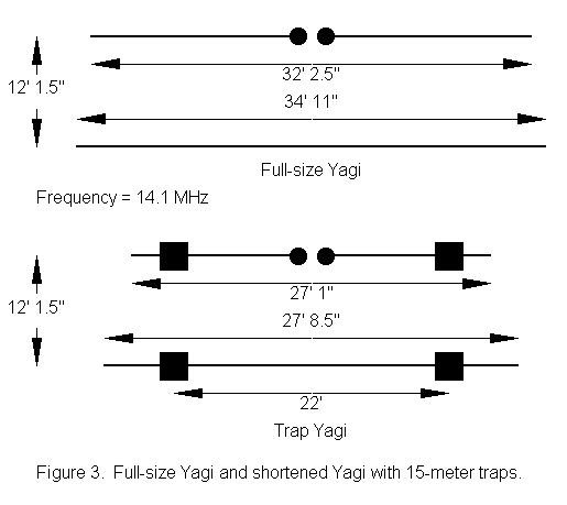
If a beam using two trapped elements could be constructed with a comparable maximum front-to-back ratio and a comparable feedpoint impedance, then the gain difference between it and the full size beam would be a good measure of gain reduction due to the shortening and other losses imposed the traps. In fact, such a beam was modeled, using the same element spacing. The driven element was 27.06' long, and the reflector was 27.7' long. The 15-meter traps were left in their original positions. It is possible that positioning the traps as they might be in a 2-band trap beam could alter the 20-meters values slightly, but the alteration was judged unlikely to be significant.

The maximum front-to-back ratio of the 14.1 MHz beam with 15-meter traps was 10.68 dB, while the feedpoint impedance was 50.5 ohms. Under these control parameters, the forward gain was 5.64 dBi. (Note: for all the 2- element beams modeled here, higher forward gains are certainly possible, but at reduced front-to-back ratios.) The gain difference between the full size Yagi and the version with 15-meter traps is 0.49 dB.

Models of tri-band beams with 3 or more elements and/or more than 2 traps per element will follow the same procedure used here for these simplified models. Data for each trap will be needed for calculations of appropriate parallel R-L-C values. Also need will be a precise element diameter schedule, along with the exact location of the traps. Although time-consuming, such modeling projects should be quite straightforward.

If the technique of modeling traps is sound, then their presence does occasion some loss in forward gain relative to trapless antennas of comparable design, at least for frequencies lower than the resonant trap frequency. How significant this loss may be is a judgment requiring the examination of factors in addition to those included in the modeling exercise. Models also suggest that at frequencies for which the traps represent resonant terminations, gain will be very similar to that of trapless versions of the antenna.

Whatever the gain situation, the exercise does demonstrate that traps can be modeled effectively as parallel R-L-C loads for each frequency of interest.

In order to ease the calculator work, I have thrown together the following GW BASIC program to calculate the properties of traps at various frequencies, based on an initial input of measured or estimated trap resonant frequency and either a. coil inductance and Q or b. coil reactance and resistance, whichever pair is known or more easily estimated. The user may refine the program as desired.

10 'trap.bas:  L. B. Cebik, W4RNL  April 1, 1997
20 CLS:PRINT "Estimating Trap Properties"
30 PRINT "L. B. Cebik, W4RNL":PRINT
40 PRINT "To estimate the properties of a trap at various frequencies, you
will need to   know or be able to estimate the following information:"
50 PRINT "  a.  The resonant frequency of the trap (normally, just below or
at the lowest       frequency of the frequency band for which it is a
trap); and either"
60 PRINT "  b.  The inductance and Q of the trap coil, or"
70 PRINT "  c.  The inductive reactance and resistance of the coil.":PRINT
100 PRINT:INPUT "Resonant frequency of trap in MHz  ";FR
110 PRINT "Coil Data:  Select the letter of the data pair you know or can
estimate.":PRINT "A.  Inductance and Q;  B.  Inductive Reactance and
Resistance"
120 A$=INKEY$:IF A$="A" OR A$="a" THEN 130 ELSE IF A$="B" OR A$="b" THEN
160 ELSE 120
130 PRINT:INPUT "Inductance in microhenries         ";L
140 INPUT "Inductor Q                         ";Q
150 XL=(6.28*FR)*L:R=XL/Q:GOTO 190
160 PRINT:INPUT "Inductive reactance in ohms        ";XL
170 INPUT "Coil resistance in ohms            ";R
180 L=XL/(6.28*FR):Q=XL/R:GOTO 190
190 C=25330/(L*(FR^2)):CB=C/1E+12
200 CLS:PRINT "Estimating Trap Properties"
210 PRINT "L. B. Cebik, W4RNL":PRINT
220 PRINT "Basic Trap Properties at Trap Resonance"
230 PRINT "Resonant Frequency ";FR;" MHz"
240 PRINT "Coil Q ";Q
250 PRINT "Coil inductance ";L;" microH"
260 PRINT "Coil reactance ";XL;" ohms"
270 PRINT "Capacitor ";C;" pF":PRINT
300 PRINT "Output Data:  Select the letter of the data type your would
like.":PRINT "A.  3 selected frequencies;  B.  Several frequencies in one
band"
310 A$=INKEY$:IF A$="A" OR A$="a" THEN 320 ELSE IF A$="B" OR A$="b" THEN
500 ELSE 310
320 INPUT "Frequency #1 in MHz               ";F1
330 INPUT "Frequency #2 in MHz               ";F2
340 INPUT "Frequency #3 in MHz               ";F3
400
XL1=6.28*(F1*L):R1=XL1/Q:N1=R1^2+XL1^2:R1P=N1/R1:XL1P=N1/XL1:FC1=F1*1000000
!:XC1=1/(6.28*(FC1*CB)):D1=XL1-XC1:IF D1=0 THEN D1=.000001
410
XN1=-(XL1*XC1)/D1:DP1=R1P^2+XN1^2:RS1=(R1P*(XN1^2))/DP1:XLS1=((R1P^2)*XN1)/
DP1:Q1=ABS(XLS1/RS1)
420
XL2=6.28*(F2*L):R2=XL2/Q:N2=R2^2+XL2^2:R2P=N2/R2:XL2P=N2/XL2:FC2=F2*1000000
!:XC2=1/(6.28*(FC2*CB)):D2=XL2-XC2:IF D2=0 THEN D2=.000001
430
XN2=-(XL2*XC2)/D2:DP2=R2P^2+XN2^2:RS2=(R2P*(XN2^2))/DP2:XLS2=((R2P^2)*XN2)/
DP2:Q2=ABS(XLS2/RS2)
440
XL3=6.28*(F3*L):R3=XL3/Q:N3=R3^2+XL3^2:R3P=N3/R3:XL3P=N3/XL3:FC3=F3*1000000
!:XC3=1/(6.28*(FC3*CB)):D3=XL3-XC3:IF D3=0 THEN D3=.000001
450
XN3=-(XL3*XC3)/D3:DP3=R3P^2+XN3^2:RS3=(R3P*(XN3^2))/DP3:XLS3=((R3P^2)*XN3)/
DP3:Q3=ABS(XLS3/RS3)
460 PRINT:PRINT"Frequency","Reactance","Resistance","Q","Para. Res."
470 PRINT F1,XLS1,RS1,Q1,R1P
480 PRINT F2,XLS2,RS2,Q2,R2P
490 PRINT F3,XLS3,RS3,Q3,R3P
495 GOTO 640
500 CLS:PRINT "Estimating Trap Properties"
510 PRINT "L. B. Cebik, W4RNL":PRINT
520 PRINT "Basic Trap Properties at Trap Resonance"
530 PRINT "Resonant Frequency ";FR;" MHz"
540 PRINT "Coil Q ";Q
550 PRINT "Coil inductance ";L;" microH"
560 PRINT "Coil reactance ";XL;" ohms"
570 PRINT "Capacitor ";C;" pF":PRINT
580 INPUT "Lowest frequency for band scan in MHz    ";FL
585 PRINT:PRINT"Frequency","Reactance","Resistance","Q","Para. Res."
590 FOR J=FL TO (FL+.5) STEP .1
600
F1=J:XL1=6.28*(F1*L):R1=XL1/Q:N1=R1^2+XL1^2:R1P=N1/R1:XL1P=N1/XL1:FC1=F1*10
00000!:XC1=1/(6.28*(FC1*CB)):D1=XL1-XC1:IF D1=0 THEN D1=.000001
610
XN1=-(XL1*XC1)/D1:DP1=R1P^2+XN1^2:RS1=(R1P*(XN1^2))/DP1:XLS1=((R1P^2)*XN1)/
DP1:Q1=ABS(XLS1/RS1)
620 PRINT F1, XLS1, RS1, Q1,R1P
630 NEXT
640 PRINT:PRINT "Press (a) for a new trap; (f) for a new frequency run; or
(q) to quit"
650 A$=INKEY$:IF A$="A" OR A$="a" THEN 10 ELSE IF A$="F" OR A$="f" THEN 200
ELSE IF A$="Q" OR A$="q" THEN 19000 ELSE 650
19000 PRINT:PRINT "To return to Main Menu, press (m)."
19001 REM c:\basic\autoend.bas
19005 M$=INKEY$:IF M$="m" OR M$="M" THEN RUN "C:\basic\menu.bas" ELSE 19005

Updated 4-2-97. © L. B. Cebik, W4RNL. Data may be used for personal purposes, but may not be reproduced for publication in print or any other medium without permission of the author.

Go to Amateur Radio Page