Last time, we looked at the basic design of high-performance 3-element Yagis. All had similar front-to-back and feedpoint impedance characteristics. They differed in gain in accord with the length of their booms. For 10-meter models, here are the design center figures as a reference for this month's investigation:

10-Meters:  28.5 MHz
Antenna Design           Free Space          Front-to-      Feed Impedance
                         Gain dBi             Back dB       R +/- jX Ohms
Long-Boom      12'       8.11                27.15          25.70 - j 0.80
Medium-Boom    10'       7.80                34.77          26.51 + j 1.69
Short-Boom      8'       7.12                41.66          27.45 - j 0.01

Each of these designs is capable of performance close to that at the design frequency across the first MHz of 10 meters. When scaled to 20 and 15 meters, the designs will cover the entire bands--and, of course, cover the WARC bands when scaled to those frequencies.

However, there is an alternative design philosophy. This philosophy sacrifices some gain in favor of wide-band characteristics. For example, the high-performance models might vary in gain by almost 0.5 dB across the span from 28 to 29 MHz. A wide-band design might vary in gain across the same span by only 0.15 dB. Likewise, a high-performance design with a feedpoint impedance in the mid-20s might just barely allow a 2:1 SWR at the band edges. A wide-band design might show those figures over the entire 10-meter band, with a corresponding shallow SWR curve within the first MHz of 10 meters.

Consequently, before we freeze our design decisions, let's look at the basic wide-band 3-element Yagi design a little more closely.

Wide-Band 3-Element Yagi Design

To create a wide-band 3-element Yagi requires more boom length for a given gain than used in the high-performance designs we surveyed last time. A 12' boom on 10 meters will yield about 1 dB less gain. What, then, is the rationale for such a design?

The fundamental reasons for going to a wide-band design are two:

1. The wide-band design provides reasonably smooth and quite adequate performance figures for the entire 10-meter band, which is 1.7 MHz wide. Hence, a single beam will cover the CW/SSB and the FM/satellite portions of the band. When scaled to 20 or 15 meters, the beam will show less change in gain, front-to-back ratio, and feedpoint impedance across those bands.

2. The wide-band design can be set for a feedpoint impedance very close to 50 Ohms, thus eliminating the need for any sort of matching network at the feedpoint. (However, a choke or 1:1 choke balun remains recommended to attenuate common mode currents.)

When these two reasons are combined, the result is a very close match to a standard 50-Ohm coaxial cable feedline with very small changes in SWR across the band of choice. This eases not only matching problems, but as well the sensitivity of some transmitting equipment to even low SWR levels that often result in automated power output reductions. Accompanying this feature is consistent gain and front-to-back ratio performance across the band.

There is an additional feature occasionally anecdotally noted by some operators. They claim superior performance results from Yagis with higher input impedances. Since these claims do not show themselves in NEC models, the vehicle we are using to evaluate performance potential, no comment can be made upon those experiences in this context.

Since the performance of wide-band models shows up most clearly on 10-meter models, we shall focus solely upon them. You can extrapolate the most relevant portions of performance curves for the other HF bands.

Two notable designs for wide-band 3-element Yagis have appeared in US antenna literature in the last decade. In the May, 1990, issue of Ham Radio, Bill Orr, W6SAI presented a wide-band design in one of his columns. In the Winter, 1998, issue of Communications Quarterly, Joe Reisert, W1JR, present a similar design, along with scalable design equations.

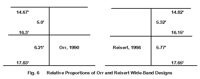
Fig. 6 shows schematically both the Orr and the Reisert designs, set for 10 meters. As we noted in connection with the high-performance designs, do NOT commit to using these dimensions to construct either design. Both are predicated on uniform diameter elements: 0.5" for the Reisert design, 1.0" for the Orr design. In common practice, Yagi elements consist of two or more sections of tubing each side of center, each section having a smaller diameter than the preceding one. This tapered-diameter schedule results in a need to lengthen elements relative to uniform-diameter models. We shall explore this topic next time.

For the moment, we want to look at the wide-band designs as concepts rather than as finished products. Both the designs require 12' booms (with allowance at each end for element-mounting hardware). The dimensions of the two antennas are sufficiently close to each other that we suspect similar performance will emerge from the antennas. And we get it.

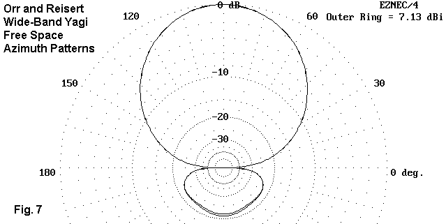
The free-space azimuth patterns in Fig. 7 overlay the Orr and Reisert designs at their resonant frequencies. The differences are too small to require comment. Gain is within 0.02 dB; front-to-back difference is less than 1 dB; and the feed point impedances are within 1 Ohm of each other at resonance. For reference, here is a handy table of values:

Antenna        Resonant       Free Space     Front-to-      Feed Impedance
               Freq. MHz       Gain dBi       Back dB       R +/- jX Ohms
Orr, 1990      28.80          7.11           21.60          47.08 + j 0.98
Reisert, 1998  28.85          7.13           20.92          46.01 + j 0.20

The slight differential in resonant frequency owes to the slight design differences, which in turn yield slightly different performance curves on 10 meters. Moving the resonant point allows one to obtain a satisfactory SWR curve across the band. We can easily sample the performance by running frequency sweeps. In the following graphs, I have used 29.5 MHz as an arbitrary upper limit in order to limit the number of data points.

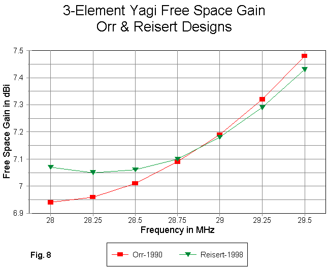
The free-space gain figures for the two designs appear in Fig. 8. The Reisert model shows the smoother gain curve, although the differences are marginal. Note that in wide-band designs, there is often a dip in the gain at the low end of the band. The dip reaches minimum for the Orr design below the lower end of 10 meters.

If we translate the first MHz of the band into roughly equivalent performance across 20 or 15 meters, the Reisert design, especially, shows a very small change in gain. The consistency of performance across the band is one of the advantages of a wide-band design.

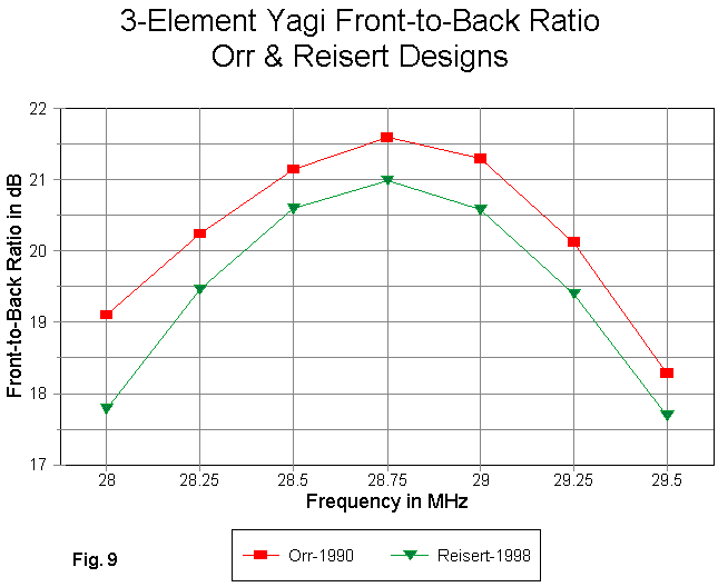
What the Orr design gives up in gain, it reacquires in front-to-back performance, as shown in Fig. 9. If we use a 20-dB front-to-back ratio as a plateau figure of merit, then the Orr design would show this across all of 20 and 15 meters. However, the Reisert design averages only about 1 dB less performance in this category, an amount unlikely to be either noticed or measurable.

With either design, the 180-degree front-to-back ratio used in the graph is a reasonable approximation of overall front-to-rear performance. The smooth rear quadrant lobe shown earlier in the azimuth patterns ensures a reasonable correlation between the 180-degree front-to-back ratio and the other two common measure of rearward performance: an averaged front-to- rear ratio and a worst-case front-to-back performance figure.

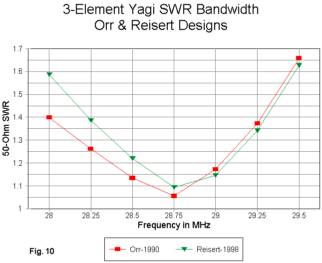
Where the wide-band designs shine is in the flatness of the SWR curves. As shown in Fig. 10, the 50-Ohm SWR curves for both designs permit a ready match directly to 50-Ohm feedline across 10 meters. If the curve centers are translated into equivalent 20 and 15 meter versions, achieving a maximum band-edge SWR of 1.35:1 is no real challenge.

For those willing to accept a slightly lower gain on the HF band of choice, the wide-band design offers consistent performance across the band with an ease of matching to 50-Ohm feedlines systems that the high-performance models cannot duplicate. The wide-band models, however, offer only the gain that the high-performance models achieve with a boom 2/3 as long.

Before we close out this preliminary survey of designs, let's take a moment to review what we are seeking to do when we decide that we want to build a 3-element Yagi.

A Pair of 2-Element Yagi Designs

Although we can design a 2-element driver-director Yagi of excellent performance and very compact size for the WARC bands, covering the wider HF bands requires that we look to 2-element driver-reflector designs. In order to see just why we might want a 3-element version, let's look at two versions of the 2-element Yagi. One uses narrow spacing, the other wide spacing.

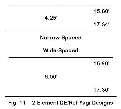
Fig. 11 shows the dimensions of both models, which use 1" uniform diameter elements. In these very standard designs, the element lengths are quite similar, with only small changes needed to accommodate the difference in boom length. At the design frequency of 28.5 MHz, the short boom is just under 1/8 wavelength long, while the long boom is somewhat over 1/6 wavelength long. At the design frequency, the modeled performance characteristics are these:

Antenna        Design         Free Space     Front-to-      Feed Impedance
               Freq. MHz       Gain dBi       Back dB       R +/- jX Ohms
Narrow Space   28.50          6.27           11.24          32.65 - j 0.32
Wide Space     28.50          6.13           10.65          51.71 + j 9.23

As the table makes clear, the design frequency gain is about 1 dB less than that of the wide-band 3-element Yagi and 2 dB less than the 12' boom high- performance version.

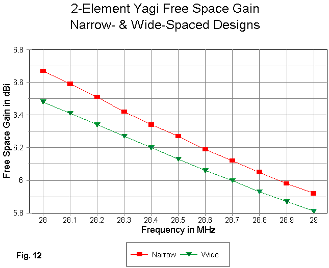
The gain curve in Fig. 12 shows that, contrary to the curves for Yagis with a director, the gain for a driver-reflector Yagi descends as the frequency increases. Were we inclined to mislead you, we might do one of two things. First, we might suggest--based on the gain value for ONLY the low end of 10 meters--that there is little difference in performance between 2- and 3-element Yagis, using either the short boom high-performance or the wide-band 3-element Yagi as a comparator. Second, using ONLY the gain value for the high end of the pass band graphed in the figure, we might try to convince you that a 3-element Yagi has an inordinately high gain advantage over the 2-element version. Both claims would be equally inaccurate. Only a graph of values over a relevant frequency range tells a full story.

With respect to the 2 2-element designs, the narrow-spaced version has the higher gain across the pass band. For this exercise, only the first MHz of 10 meters is shown, although the wide-spaced version will be usable across the entire 10-meter band.

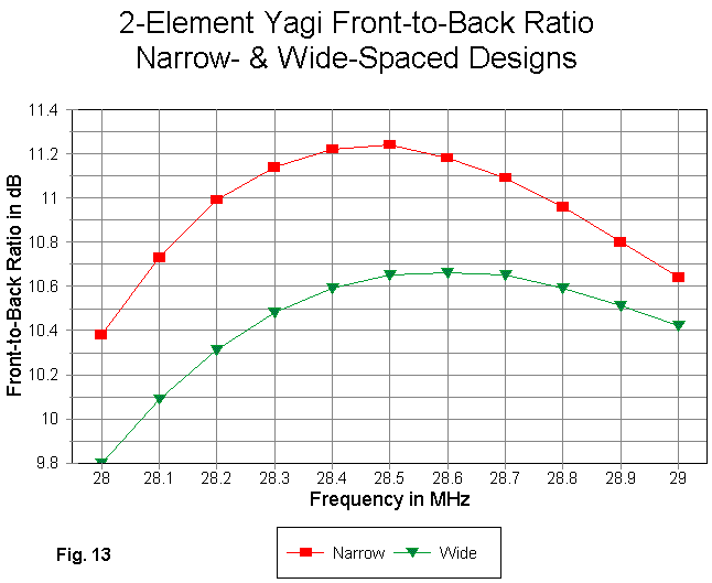
The overall front-to-back ratio of a 2-element driver-reflector Yagi is fairly weak, failing to reach 12 dB as shown in Fig. 13. (Note: this weaker front-to-back ratio can be an advantage in certain kinds of net and contest operations where total exclusion of signals from the rear quadrants can be a hindrance to efficient operation.) The narrow-spaced version has the stronger values, but the curve is clearly sharper than the gentler slope of the values for the wide-spaced version. The wide-spaced model front-to-back ratio is about 10 dB at the upper limit of the 10-meter band.

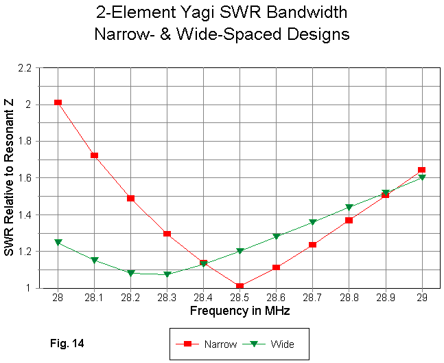
The SWR curves in Fig. 14 for the two models tell different stories. The sharp curve for the narrow-spaced model has a resonant point of about 32.5 Ohms. Hence, the antenna will require a matching network for a 50-Ohm main feedline. In contrast, the curve for the wide-spaced model is based on 50 Ohms. The curve has been intentionally shifted downward in frequency to show the shallow rise in value above the lowest value. By moving the center point of the curve upward in frequency simply by shortening the driver element slightly, the SWR can be held below 2:1 across the entire 10-meter band. This permits direct matching to a coax line with no matching network needed (but with the recommended choke or choke balun in place, as always).

With the 2-element Yagi curves in mind, we can make more precise our reasons for wanting to move to a 3-element Yagi.

1. Most prominently, for operations that need it, the front-to-back values for all versions of the 3-element Yagi are considerably superior to those of the 2-element driver-reflector Yagi.

2. The gain of a high-performance, long-boom 3-element Yagi show about a 2 dB advantage over the 2-element Yagis. This amount of gain is significant. The short-boom and the wide-band 3-element Yagis show about half that value of extra gain, and the significance of the difference is reduced accordingly.

3. Both 2- and 3-element Yagis can be designed for 50-Ohm feedpoint impedances that hold up even across the wide reaches of 10-meters. However, in both 2- and 3-element designs, narrower spacing allows more gain per unit-length of boom.

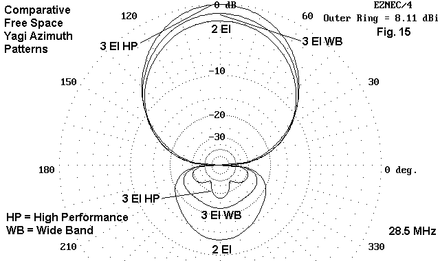
Fig. 15 shows comparative free-space azimuth patterns for the narrow-spaced 2-element Yagi, the wide-band 3-element Yagi, and the 12' boom high-performance Yagi. The steps of performance improvement are clear in the graphic. What the patterns cannot show is that, where narrower band operation and a 25-Ohm feedpoint impedance are acceptable, the short-boom 3-element Yagi will provide roughly the same gain and front-to-back ratio as the wide-band model with 2/3 the boom length.

In the end, the final decision as to which design meets our needs will use some mixture of the performance figures, plus a measure of the physical properties of the structure we propose to build. Hence, every such decision will be very individualized. The various models we have presented are intended only to provide some comparative measures as a background against which to make the final decision.

Still, we have not addressed some of the structural considerations that go into the decision. Boom length so far is a matter of a number, not a real physical property. As well, we need to look at what real tapered-diameter elements may imply for the antenna design. Both of these questions mean that we shall have to add a "Part 3" to this series--next time.

Updated 07-31-99. © L. B. Cebik, W4RNL. This item appeared in AntenneX, May, 1999. Data may be used for personal purposes, but may not be reproduced for publication in print or any other medium without permission of the author.

Go to Part 3: What Real Dimensions Shall I Use?

Return to Index