
 A 10-Meter LPDA
To leave behind the wide-band Yagi using open-sleeve coupled drivers with only a basic design would be incomplete. The antenna deserves to be interrogated with respect to some of the same questions we posed of the LPDA. Most of the relevant questions have to do with element diameter, and the answers may bring us full circle in a special way.
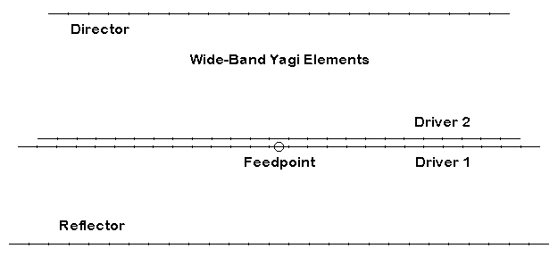
As a reference, the sketch above designates the parts of our wide-band Yagi design. Driver 1 is directly fed, while Driver 2 is open-sleeve coupled to Driver 1. The result is a wide band Yagi capable of covering all of 10 meters with performance that approaches the earlier 4-element 75-Ohm line LPDA. With respect to our initial specifications, free space gain is a tiny bit lower than 7 dBi at the lower end of the band and the front-to- back ratio does not quite reach 20 dB at the band edges. However, the savings in weight and construction complexity might well offset these minor deficiencies.
To check the degree to which element diameter might alter the Yagi performance, I changed from the initial 0.5" elements to 1" elements. This required changing virtually all of the element lengths and positions to achieve a model with essentially the same coverage and flat SWR curve. The results appear in the table below, which sets the 0.5" and 1.0" element models side by side. Once more, the modeling is done in MININEC (AO), because the close spacing of the 0.5" diameter drivers yields slightly erroneous reports in NEC-4.
4-Element Wide-Band Yagi
Free Space Symmetric       28.75 MHz              4 6060-T6 wires

Element Diameter (Inches)      0.5                      1.0
Reflector length              212.50                   212.50
Driver 1 length               205.50                   209.00
Driver 2 length               189.50                   188.00
Director length               180.80                   178.00
Spacing from Reflector
Driver 1                       39.50                    37.75
Driver 2                       43.50                    44.75
Director                       95.50                    95.75

28.000 MHz:   Impedance        52.7 - j 8.0            48.4 - j 5.1
              SWR              1.18                    1.11
              Wire Losses      0.03 dB                 0.01 dB
              Efficiency       99.4%                   99.7%
              Forward Gain     6.90 dBi                6.99 dBi
              F/B              18.53 dB                19.86 dB

28.250 MHz:   Impedance        53.0 - j 8.9            47.7 - j 4.5
              SWR              1.20                    1.11
              Wire Losses      0.03 dB                 0.01 dB
              Efficiency       99.4%                   99.7%
              Forward Gain     6.87 dBi                6.99 dBi
              F/B              20.69 dB                22.63 dB

28.500 MHz:   Impedance        52.1 - j 8.3            46.4 - j 2.6
              SWR              1.18                    1.10
              Wire Losses      0.03 dB                 0.02 dB
              Efficiency       99.3%                   99.6%
              Forward Gain     6.88 dBi                7.02 dBi
              F/B              23.09 dB                26.44 dB

28.750 MHz:   Impedance        50.9 - j 6.3            45.2 + j 0.4
              SWR              1.13                    1.11
              Wire Losses      0.03 dB                 0.02 dB
              Efficiency       99.3%                   99.6%
              Forward Gain     6.93 dBi                7.08 dBi
              F/B              26.06 dB                33.24 dB

29.000 MHz:   Impedance        50.4 - j 3.6            44.8 + j 3.8
              SWR              1.07                    1.15
              Wire Losses      0.03 dB                 0.02 dB
              Efficiency       99.2%                   99.6%
              Forward Gain     7.02 dBi                7.17 dBi
              F/B              28.49 dB                35.24 dB

29.250 MHz:   Impedance        51.2 - j 1.4            45.5 + j6.8
              SWR              1.04                    1.19
              Wire Losses      0.04 dB                 0.02 dB
              Efficiency       99.1%                   99.5%
              Forward Gain     7.14 dBi                7.27 dBi
              F/B              25.74 dB                26.27 dB

29.500 MHz:   Impedance        52.9 - j 2.1            47.1 + j 7.6
              SWR              1.07                    1.18
              Wire Losses      0.05 dB                 0.02 dB
              Efficiency       98.9%                   99.4%
              Forward Gain     7.28 dBi                7.40 dBi
              F/B              21.03 dB                21.23 dB

29.750 MHz:   Impedance        51.4 - j 9.0            47.2 + j 3.6
              SWR              1.20                    1.10
              Wire Losses      0.06 dB                 0.03 dB
              Efficiency       98.6%                   99.3%
              Forward Gain     7.44 dBi                7.53 dBi
              F/B              17.10 dB                17.73 dB

30.000 MHz:   Impedance          36.5 - j 16.6         37.7 - j 3.5
              SWR                 1.64                 1.34
              Wire Losses         0.10 dB              0.05 dB
              Efficiency         97.7%                 98.9%
              Forward Gain        7.59 dBi             7.65 dBi
              F/B                13.87 dB              15.07 dB
Although the element lengths do not require very large changes, the spacing of the drivers between the limits set by the 8' boom does change significantly. Driver 1 is 1.75" close to the reflector, while Driver 2 is 1.25" closer to the director in the 1.0" diameter model. The net spacing between driven elements increases by 3.0", which nearly doubles the spacing relative to the half-inch model. The most notable element length change is the increase in Driver 1, which was necessary to accommodate the spacing changes and still yield a satisfactory SWR curve and curves that parallel those for the smaller diameter model.
Although the essential data appears in the table, separating each category of information may provide further insight into the two models.
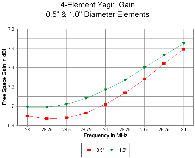
The gain curves for the two models show a small increase for the 1.0" model relative to the 0.5" model. The average increase across the band is about 0.11 dB, which is numerically noticeable, but not very significant operationally. Even this size increase may not be typical for all increments of difference one might choose for making the comparison. We shall return to this point when we later look at tapered-diameter elements.
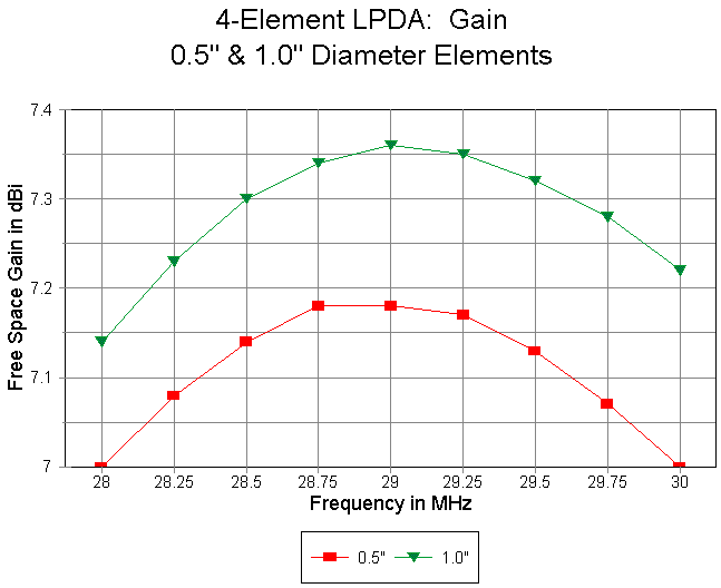
For comparison, we may plot the gain curves of optimized 75-Ohm antenna transmission line 4-element LPDAs, using the 0.5" and the 1.0" element sizes. The curve above shows the results. Between the two element sizes, the average gain differential is about 0.18 dB, about one and two-thirds the difference for the Yagi (and, as we shall see, the Yagi figures may be artificially high). Although one case does not prove a general point, the results are indeed suggestive for monoband LPDAs: element diameter does have a noticeable impact on overall antenna gain across the limited passband of a monoband antenna.
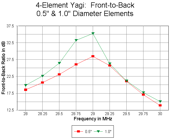
With respect to the front-to-back ratio of a wide-band Yagi of the design we are exploring, the difference in element diameter has less of an impact at the band edges than it does on the peak front-to-back ratio (recorded here as the 180-degree ratio). The peak in the front-to-back ratio of the model using fatter elements, which occurs at about 29.85 MHz, would not in itself be a sufficient reason for selecting that model over the one using smaller elements.
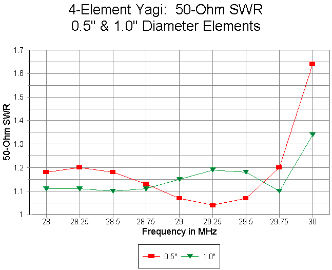
The comparative 50-Ohm SWR curves for the two antennas permits us to put some factors into perspective. Within the 10 meter band from 28 to 29.7 MHz, both antennas provide SWR values no greater than 1.2:1, with climbing values above the upper band edge. In practical terms, neither antenna outperforms the other.
However, notice the differences in the undulations of the curves across the band. They reflect some of the less precise points of designing a wide-band Yagi using open-sleeve coupled drivers. Slightly different lengths and spacing chosen for the drivers, in their interactions with the reflector and director can produce differently shaped SWR curves for essentially the same gain and front-to-back figures. Since there is only one reflector and one director, each will favor a frequency region (at the low end for the reflector and at the upper end for the director), with some territory resting upon the balance of the two drivers together. Slight changes to any element can change the favored region of lowest SWR. These changes also tend to move the gain and front-to-back curves up and down the band, and usually the designer will compensate by changing the dimension of a different element to bring the curve back into the desired full-band coverage. The result will be some variance in the undulations of the SWR curve from one design to another, designs that achieve just about the same gain and front- to-back figures.
The upshot is that for the wide-band Yagi, element diameter has far less an impact on overall performance than it does for the monoband LPDA. While the LPDA seemed to benefit from the use of larger diameter elements, the Yagi shows only such marginal improvements as may be offset by the increase in weight of the larger elements.
I selected 0.625" inner element sections, 72" long (or 36" either side of center). The ends are 0.5" diameter tubes. As expected, the shift to tapered-diameter elements required a total redesign of the antenna dimensions. The results, as modeled in MININEC (AO), appear in the table below.
4-Element Wide-Band Yagi
Free Space Symmetric       28.75 MHz              4 6060-T6 wires

Element Type                  Uniform             Tapered-Diameter*
Element Diameter (Inches)      0.5                     0.625/0.5
Reflector length              212.50                   215.50
Driver 1 length               205.50                   207.20
Driver 2 length               189.50                   191.80
Director length               180.80                   182.60
Spacing from Reflector
Driver 1                       39.50                    37.75
Driver 2                       43.50                    45.00
Director                       95.50                    96.00
(*Note:  0.625" portion = 72" centered)


28.000 MHz:   Impedance        52.7 - j 8.0            52.3 - j 8.4
              SWR              1.18                    1.19
              Wire Losses      0.03 dB                 0.02 dB
              Efficiency       99.4%                   99.5%
              Forward Gain     6.90 dBi                6.95 dBi
              F/B              18.53 dB                19.08 dB

28.250 MHz:   Impedance        53.0 - j 8.9            52.4 - j 8.0
              SWR              1.20                    1.18
              Wire Losses      0.03 dB                 0.02 dB
              Efficiency       99.4%                   99.5%
              Forward Gain     6.87 dBi                6.94 dBi
              F/B              20.69 dB                21.63 dB

28.500 MHz:   Impedance        52.1 - j 8.3            51.3 - j 6.1
              SWR              1.18                    1.13
              Wire Losses      0.03 dB                 0.02 dB
              Efficiency       99.3%                   99.4%
              Forward Gain     6.88 dBi                6.96 dBi
              F/B              23.09 dB                24.80 dB

28.750 MHz:   Impedance        50.9 - j 6.3            49.9 - j 2.7
              SWR              1.13                    1.06
              Wire Losses      0.03 dB                 0.03 dB
              Efficiency       99.3%                   99.4%
              Forward Gain     6.93 dBi                7.02 dBi
              F/B              26.06 dB                29.54 dB

29.000 MHz:   Impedance        50.4 - j 3.6            49.1 + j 1.6
              SWR              1.07                    1.04
              Wire Losses      0.03 dB                 0.03 dB
              Efficiency       99.2%                   99.4%
              Forward Gain     7.02 dBi                7.11 dBi
              F/B              28.49 dB                32.97 dB

29.250 MHz:   Impedance        51.2 - j 1.4            49.5 + j6.1
              SWR              1.04                    1.13
              Wire Losses      0.04 dB                 0.03 dB
              Efficiency       99.1%                   99.3%
              Forward Gain     7.14 dBi                7.22 dBi
              F/B              25.74 dB                26.59 dB

29.500 MHz:   Impedance        52.9 - j 2.1            51.6 + j 9.2
              SWR              1.07                    1.20
              Wire Losses      0.05 dB                 0.04 dB
              Efficiency       98.9%                   99.2%
              Forward Gain     7.28 dBi                7.36 dBi
              F/B              21.03 dB                21.38 dB

29.750 MHz:   Impedance        51.4 - j 9.0            54.5 + j 7.2
              SWR              1.20                    1.18
              Wire Losses      0.06 dB                 0.05 dB
              Efficiency       98.6%                   99.0%
              Forward Gain     7.44 dBi                7.50 dBi
              F/B              17.10 dB                17.69 dB

30.000 MHz:   Impedance          36.5 - j 16.6         49.5 - j 3.0
              SWR                 1.64                 1.06
              Wire Losses         0.10 dB              0.07 dB
              Efficiency         97.7%                 98.5%
              Forward Gain        7.59 dBi             7.63 dBi
              F/B                13.87 dB              14.86 dB
The increase in element lengths is about as expected. More noticeable is the change in driver spacing relative to the uniform 0.5" model, with Driver 1 moved toward the reflector and Driver 2 moved toward the director. In fact, the spacing (and to some degree, the element lengths) are closer to those required by the uniform 1.0" model. Once more, we can look at the data more closely by separating it into categories.
The gain curves are congruent, with the tapered model showing a slight increase in gain over the untapered model. The amount of the increase is operationally insignificant. However, the gain of the tapered-element model is also insignificantly different from the gain of the uniform 1.0" diameter model. Given the similarities of driver spacing between the tapered and fat element design, it is likely that the lower gain of the 0.5" is the more abberant result, stemming from the required closer spacing of drivers. (See the notes near the end on the SWR curve for NEC-4 for related findings.)
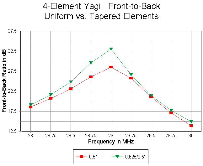
The front-to-back ratio curve of the tapered-diameter model has a more distinct peak than that of the uniform-diameter model. Because the net increase in element size is so small, the more likely source of the front- to-back peak is the alteration of the driver spacing. With spacing that is close to that used for the 1" model, the tapered-diameter model shows a peak that also resembles the one obtained for the larger diameter element model. As expected, band-edge performance is not greatly affected by the presence of the peak.
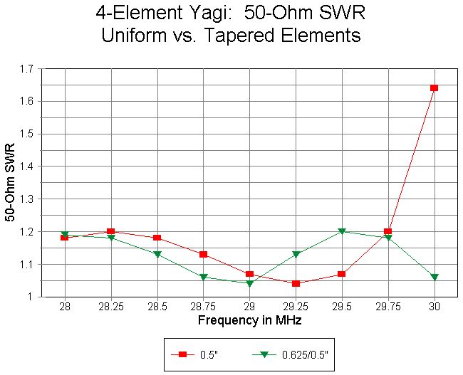
For the tapered-diameter element model, the SWR curve shows a value of 1.2:1 or less not only across the 10-meter band, but above 30 MHz as well. I described the design situation that yields undulations of various types. The new model has simply compressed the undulations for two peaks within the passband of the model. The other models used so far have had a single peak, with the second one trailing off beyond the band edge.
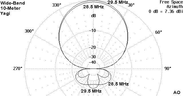
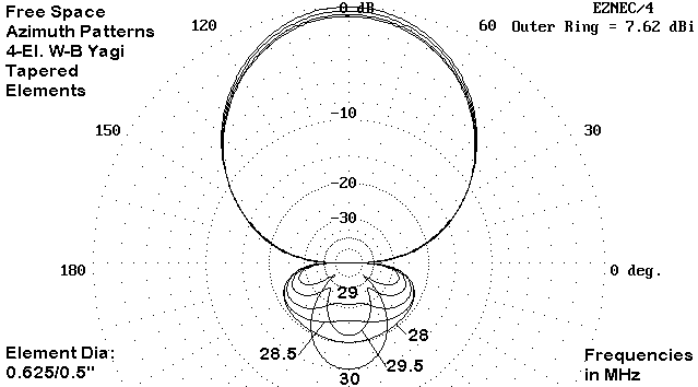
Regardless of slight peaks and valleys in the SWR curve, the tapered- diameter design appears to be a complete success within the overall limitations of the antenna configuration. The representative free space azimuth patterns (shown within the AO limit of two patterns overlaid) reveal well-behaved forward and rearward lobes that meet our standard expectations of Yagi designs.
It seemed reasonable to transport the MININEC model back to NEC-4 (using EZNEC Pro) and see what might result by way of reports. The following graphs compare the MININEC numbers with those of NEC-4. Since NEC-4 is sensitive to tapered diameter elements to a small degree (but no where to the degree of NEC-2), I ran the model first with no Leeson correction factor. Then I reran the model invoking the Leeson corrections that transform tapered-diameter elements into substitute uniform-diameter elements with the same electrical properties. The results of invoking the correction factor will be coincide with those of using the same correction factors in NEC-2, since uniform-diameter elements yield the same results in both levels of NEC.
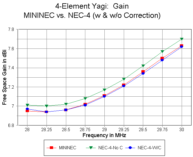
The gain curves are instructive. If the close spacing of the elements had any remnant affect on the gain report, it would show up in the corrected curve, since the Leeson correctives do not affect the close-spacing sensitivity of the program. However, the corrected curve for NEC-4 and the MININEC curve are coincident from one end of the passband to the other. The uncorrected NEC-4 curve shows slightly higher gain figures as a result of the still imperfect handling of tapered-diameter elements.
(This account is incomplete. It is possible, but unlikely, that the thinner uniform-diameter elements used in the Leeson corrections, which range from 0.538" to 0.55", might have a very slight positive affect in reducing the close-spacing sensitivity of uncorrected NEC-4 beyond the wider spacing used in the model. The net diameter difference of about 0.07" has a very low probability of showing any gain over-reportage on its own. However, to decisively establish this as fact would require one to separate the effects of element spacing completely from the effects of element diameter changes, which is not practical in this context.)
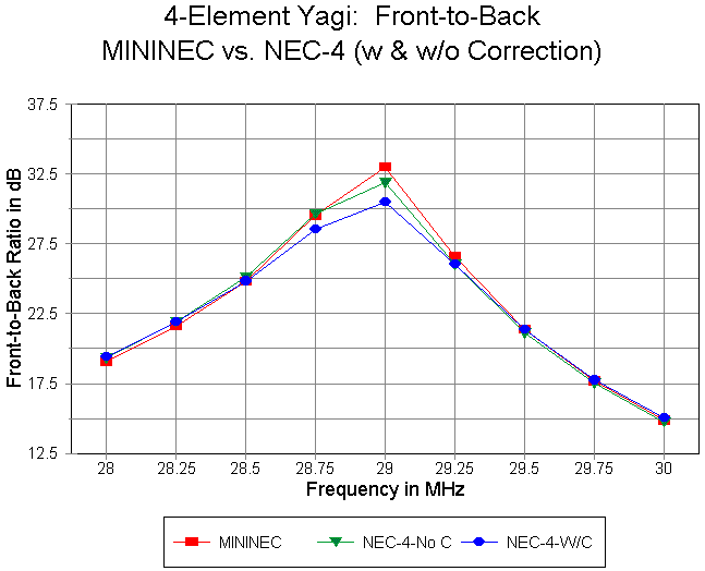
The front-to-back curves are insignificantly different. Although there might be a slight difference in the ultimate peak value, the curve indicates that most of the difference is due to a slight difference in reported frequency of the peak (as indicated by the changing slope of the lines leading to the reported peak value in the sampling). Nothing in these curves can suggest that any one modeling system is more authoritative than any other.
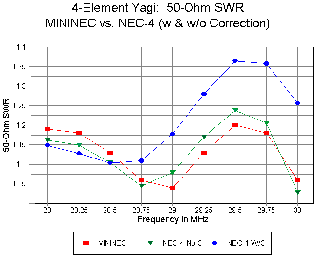
The 50-Ohm SWR curves for the three model runs are most interesting. The uncorrected NEC-4 curve most closely coincides with the MININEC curve. This raises the question of why the corrected NEC-4 curve departs from the others by a noticeable amount--even if the amount still yields a report of outstanding wide-band performance in this category of concern.
Part of the answer lies in the Leeson correctives themselves as they are applied to open-sleeve coupling models. The substitute elements produced by the corrective range in diameter from 0.538" to 0.55", with the Driver 1 having a diameter of 0.541" and Driver 2 having a diameter of 0.55". These diameters are smaller than the center 0.625" diameter of the 2 drivers. Although the Leeson correctives can capture the relatively correct source impedance at the low end of the band, when the directly-fed driver dominates, the source impedances reports by the corrective at the upper end of the band indicate a drop in source resistance, as we might well expect of thinner elements with the prescribed spacing. Although the amount of difference in coupling between the master and slave drivers is too small to materially affect the gain and front-to-back ratio figures, the impedances at element centers differ enough to show up in the source resistance and 50-Ohm SWR numbers. This is not fault of the Leeson correctives, since they were never designed to cover open-sleeve coupling situations.
One of the motivations for checking the performance of NEC-4 on the tapered-diameter model grew from a desire to check a large number of free space azimuth pattern simultaneously (AO is limited to 2).
Since we have established the general reliability of corrected NEC-4 with respect to gain and front-to-back ratio, the azimuth patterns collected in the above figure can be considered reliable guides to expectations you may have from the wide-band open-sleeve coupled Yagi.
Second, we have had a chance to compare Yagis and LPDAs with respect to the question of the influence of element diameter. Unless some contrary evidence emerges, the results tell me to expect much less difference in performance from Yagis using elements of different diameter than from LPDAs with the same range of variation. What we suspected early in this inquiry has received some further (but far from final) confirmation.
Third, we learned that the original 0.5" wide-band model of a Yagi for 10 meters was no fluke--that it can be replicated in a large range of material diameters and tapers with due attention to element length and spacing. The optimizing process may be a bit slower than for simple Yagis (which are amenable to automated processes), but results are assured. That factor alone is worth the time of investigation, because it converts question into confidence. One can now listen to the voice that whispers, "Build it. It will work."
However, that was the same voice I heard when I reached a similar point in
looking at the monoband 4-element LPDA. Both appear to be highly promising
designs that come as close as possible, each in its own way, to meeting the
criteria set for this project.
Updated 11-18-98. © L. B. Cebik, W4RNL. Data may be used for
personal purposes, but may not be reproduced for publication in print or
any other medium without permission of the author.